Literature review: ODE Stability

AIM: To understand numerical methods used to solve Ordinary Differential Equations and the stability of these methods.

Introduction:

Ordinary Differential Equations are used extensively in physics, and solving them becomes vital, in order to understand the behaviour of a particular system. Many ordinary differential equations are complex in nature, and obtaining their analytical solutions becomes difficult, depending on the complexity of the ODE. Obtaining these solutions are time consuming in nature. In order to obtain solutions at a faster pace, numerical approximations are obtained by employing Numerical Methods.

Theory:

Numerical methods are used to obtain approximate solutions for ordinary differential equations. Numerical methods can be catagorised into two basic types:

(1) One step methods.

(2) Linear multistep methods.

The main difference between these methods are the number of steps and the number of points used to obtain the numerical approximation of the solution. Using an increased number of points has some benefits over using a single point. The Adams-Bashforth method and the Adams-Moulton methods are examples of linear multistep methods, while the forward and backward Euler methods are examples of one step methods.

These methods can be further catagorised into explicit, implicit and semi-implicit methods.

(a) Explicit method:

An explicit method utilizes the values at the current step to calculate the solution at the next step. This method is the simplest to implement, and will be discussed in the sections below.

The Forward difference Euler method is a first order method.

The Runge-Kutta 4th order method has error of the 4th order, and the results obtained by this method should be highly accurate. However, this method is explicit in nature, and the stability of this method will be compared to the rest of the methods.

(i)Forward difference Euler method:

`y[i] = y[i-1] + dt*(f(t[i-1],y[i-1])`

`y' = dy/dt= f(t,y)`

`dt` = time step

`i =`node point

(ii) Runge-Kutta 4th order method:

`k1[i] = dt*(f(t[i-1],y[i-1]))`

`k2[i] = dt*(f(t[i-1] + dt/2)),``(y[i-1] + (k1[i])/2))`

`k3[i] = dt*(f(t[i-1] + dt/2)),``(y[i-1] + (k2[i])/2))`

`k4[i] = dt*(f((t[i-1] + dt),``(y[i-1]+k3[i])))`

`y[i] = y[i-1] + (1/6)*(k1[i]+(2*k2[i])+(2*k3[i])+k4[i])`

`y' = dy/dt= f(t,y)`

`dt` = time step

`i =`node point

(b) Implicit method:

An implicit method, and utilizes both, values calculated on the next time step, and the current time step, in order to obtain the numerical approximation of the solution. The benefits of using an implicit method will be discussed in the sections below. For this literature review, first order and second order approximation methods have been used for understanding the factors that stability depends on.

The backward diference Euler method is a first order method, and the Trapazoid method is a second order method.

(i)Backward difference Euler method:

`y[i] = y[i-1] + dt*(f(t[i],y[i])`

`y' = dy/dt= f(t,y)`

`dt` = time step

`i =`node point

(ii)Trapazoidal method:

`y[i] = y[i-1] + (dt/2)*(f(t[i-1],y[i-1])) -f(t[i],y[i]))`

`y' = dy/dt= f(t,y)`

`dt` = time step

`i =`node point

(c) Semi-implicit method:

The semi-implicit method uses explicit and implicit methods to obtain the numerical approximation of the solution. The Crank-Nicholson method is an example of this type of method. This will not be discussed in this literature review.

Derivative of the function being used:

`y' = -(1000*y) -( e^(-1*t))`

Stability conditions:

The following stability conditions have been used in the program. These stability conditions have been derived for each numerical method(except for R-K 4th order,which will not be covered in this project), and have been shown in the Results section of this report.

(i)Forward difference Euler method:

Forward difference Euler stability function`= 1 - 1000*dt`

(ii)Backward difference Euler method:

Backward difference Euler stability function `= (1/(1+1000*dt))`

(iii)Trapezoidal method:

Trapezoidal method stability function `= (1-500*dt)/(1+500*dt)`

Coding approach:

The following steps were taken in order to achieve the numerical approximations using the different methods listed above:

Step I: Importing libraries and setting values for time,and time step.

• The numPy and matplotlib libraries are imported into the program by using the 'import' command.
• The start and end times of the solution are defined, along with the time step size required. The time step size is in list format, in order to accomodate multiple values.

Lines of code:

import numpy as np
import matplotlib.pyplot as plt

t_start = 0
t_end = 0.1
dt = [0.0001,0.0005,0.001,0.002,0.01]

Step II: Defining functions

This step involves defining functions for all of the numerical methods mentioned above and the derivative of the function(y').

(i) Defining dy/dt :

• The function for the derivative is defined with the command 'def' and is given an appropriate name, with the input arguments set as the time step of the simulation(t) and the numerical approximation of the solution at that particular time step(y).
• The return value is set as the derivative mentioned in the theory section. The 'exp' function of the numPy library is used to define the exponent term in the derivative.

Lines of code:

#The derivative of the ODE(y'):
def f(t,y):
	return -1000*y - np.exp(-1*t)

(ii) Defining Explicit and implicit functions:

• The function for the derivative is defined with the command 'def' and is given an appropriate name,with the input arguments set as the simulation start and end times(t_start and t_end) and the time step size.
• The 'arange' function of the numPy library allows us to obtain a range of values for time 't', using the time step size as the interval between two consecutive values, and allows the use of a float value.
• The function 'len' is used to obtain the total number of time steps.
• Time step and the numerical approximation of the solution of the ODE(y), are defined as local variables.
• The initial value of the numerical approximation of the solution of the ODE, 'y', is set as a list of zeroes using the 'zeros' function, and the number of zeroes is set, is the same as the number of time steps being computed in the numerical approximation. This has been done in order to create a list that can accomodate the required values of 'y', over every time step. The zeroes are eventually replaced with the values that will be computed within the functions of the different numerical methods defined within them.
• Since the first value of the list that has been created is zero, that value will be for calculating the first value of 'y' for the first time step. After the first value is computed, the next value in the list of zeroes will be replaced with this new value, and this new value will be used for computing the next time step. A list is a mutable data type, and this technique can be used for this case.
• This technique has been used for both,the implicit and explicit functions.

(A) Explicit methods:

(a) Explicit: Euler forward difference method:

• A 'for' loop is set with the range identical to the number of time steps over which the simulation is being run. This has been done using the 'len' function, and the 'arange' function of the numPy library.
• Within the 'for' loop, the function for the forward difference method is specified.
• The stability condition for the explicit method is inserted into the function as well.
• The function is set to return lists for 't' and 'y'.

Lines of code:

#Explcit: Euler Forward difference method
def explicit_euler(t_start,t_end,dt):
	t = np.arange(t_start,t_end,dt)
	y = np.zeros(len(t))
	for i in np.arange(1,len(t)):

		y[i] = y[i-1]  + dt*(f(t[i-1],y[i-1]))

	Euler_stability = 1 - 1000*dt
	print('The stability value of the forward difference Euler method is',str(Euler_stability),'.')
	return [t,y]

(b) Explicit: Runge-Kutta 4th order method:

This method utilizes four steps, one for the initial time step, two for the mid-point and one for the end time step.

• A list of zeroes the size of the total number of time steps are created for the increments k1,k2,k3 and k4. This works the same way as 'y', mentioned in the previous method. A 'for' loop is set with the range identical to the number of time steps over which the simulation is being run is created, with the formulae(shown in the theory section) for k1,k2,k3,k4 and y set within it.
• The value of k1 is calculated using the values of 't' and 'y' of previous time step, and is inserted in k2. Similarly k2 is inserted into k3 and k3 is finally inserted into k4. All of these values are then used to obtain the numerical approximation of the ODE solution.
• The function is set to return lists for 't' and 'y'.

Lines of code:

#Explicit: Runge-Kutta fourth order
def explicit_RK_4(t_start,t_end,dt):
	t = np.arange(t_start,t_end,dt)
	y = np.zeros(len(t))

	k1 = np.zeros(len(t))
	k2 = np.zeros(len(t))
	k3= np.zeros(len(t))
	k4 = np.zeros(len(t))

	for i in np.arange(1,len(t)):
		k1[i] = dt*(f(t[i-1],y[i-1]))
		k2[i] = dt*(f((t[i-1] + (dt/2)),(y[i-1] + ((k1[i])/2))))
		k3[i] = dt*(f((t[i-1] + (dt/2)),(y[i-1] + ((k2[i])/2))))
		k4[i] = dt*(f((t[i-1] + dt),(y[i-1]+k3[i])))
		y[i] = y[i-1] + (1/6)*(k1[i]+(2*k2[i])+(2*k3[i])+k4[i])

	return [t,y]

(B) Implicit methods:

• These methods utilize the values of 't' and 'y' of the next time step to compute the slope(dy/dt), and the value of 'y' at the current time step, to find the numerical approximation of the solution of the next time step.
• However, using the formulae shown in the theory section does not translate well into a program, as the values of the next time step and the current time step must be kept separate in order to obtain the next time step. Hence, the formulae have been manually changed in order to run it in a program.

The following formulae have been used to obtain the value of 'y' in the next time step:

(a) Implicit: Euler backward difference method

`y[i] = ((-dt*e^(-t[i])) + y[i-1])/(1+1000*dt)`

(b) Implicit: Trapezoid method

`y[i] = (y[i-1] + (dt/2)*(f(t[i-1],y[i-1])) - ((dt/2)*e^(-t[i])) )/(1+(500*dt))`

• Both of these methods operate the same way. A 'for' loop is set with the range identical to the number of time steps over which the simulation is being run, and the formulae shown above are inserted into the loop.
  
• The stability conditions for both implicit methods have been inserted into their respective functions.
• The functions return a list of the values of 't' and 'y'.

Lines of code:

#Implicit: Euler Backward Difference Method
def implicit_euler(t_start,t_end,dt):
	t = np.arange(t_start,t_end,dt)
	y = np.zeros(len(t))
	for i in np.arange(1,len(t)):

		y[i] = (-dt*np.exp(-t[i]) + y[i-1])/(1+1000*dt)

	Implicit_euler_stability = (1/(1+1000*dt))
	print('The stability value of the backward difference Euler method is',str(Implicit_euler_stability),'.')
	return [t,y]

#Implicit: Trapezoidal Method
def implicit_trapezoid(t_start,t_end,dt):
	t = np.arange(t_start,t_end,dt)
	y = np.zeros(len(t))
	for i in np.arange(1,len(t)):

		y[i] = (y[i-1] + (dt/2)*(f(t[i-1],y[i-1])) - ((dt/2)*np.exp(-t[i])) )/(1+(500*dt))

	Trap_stability = (1-500*dt)/(1+500*dt)
	print('The stability value of the Trapazoidal method is',str(Trap_stability),'.')

	return [t,y]

(C) Analytical solution:

The analytical solution of the ODE has been displayed below.

Analytical solution `= (e^(-1000*t)*(1-e^(999*t)))/999`

• Similar to the steps mentioned above, a function for the analytical solution of the ODE is defined, with the input arguments set as the simulation start and end times(t_start and t_end) and the time step size.
• The formulae for the analytical solution is inserted within the function, and is set to return the analytical solution at a particular time step.

Lines of code:

#Actual solution:
def analytical_sol(t_start,t_end,dt):
	t = np.arange(t_start,t_end,dt)
	act_sol = (np.exp(-1000*t)*(1-np.exp(999*t)))/999

	return act_sol

Step III: Running functions and plotting commands

• A 'for' loop is created, using the list of the time step size values mentioned in the first step. This will allow us to observe the effect of time time step size on the numerical methods.
• The time step size is printed to the console window for reference.
• The functions for the numerical approxiations are run using the input arguments listed in Step II(ii)(start time and end time of the simulation, as well as the time step size of the required range of time steps). The time steps are associated with the functions as the functions are meant to return both 't' and 'y' values over said time steps in list form, and is nescessary to pair 't' with 'y'.
• The analytical function returns the analytical solution.
• Finally, the plot is created for time steps vs numerical approximation of the solution and time steps vs analytical solution.

The following functions in the matplotlib library were used to create the plot mentioned above.

1. xlabel, ylabel : Used to name the X and Y axes respectively.
2. plot : Used to produce a line plot for time steps vs numerical approximation of the solution and time steps vs analytical solution, and specifying the method time and color of the line by using 'label' and 'color' respectively.
3. legend : Used to display the legend.
4. show : Used to display the plot. This is kept outside the 'for' loop, so that all of the plots for different time step size values are displayed.

Lines of code:

for dt in dt: 
	print('n')
	print('Time step size = '+str(dt)+'s')
	t,y_explicit = explicit_euler(t_start,t_end,dt)
	t,y_explicit_RK_4 = explicit_RK_4(t_start,t_end,dt)
	t,y_implicit = implicit_euler(t_start,t_end,dt)
	t,y_implicit_trapezoid = implicit_trapezoid(t_start,t_end,dt)
	act_sol  = analytical_sol(t_start,t_end,dt)

	plt.figure()
	plt.title('Time step vs ODE solution(Time step size ='+str(dt)+')')
	plt.xlabel('Time(t)')
	plt.ylabel('Numerical solution of the ODE')
	plt.plot(t,y_explicit,color = 'r',label= 'Explicit Euler Forward Difference method')
	plt.plot(t,y_explicit_RK_4,color = 'g',label= 'Explicit Runge-Kutta fourth order method')
	plt.plot(t,y_implicit,color = 'b',label= 'Implicit Euler Backward Difference method')
	plt.plot(t,y_implicit_trapezoid,color = 'm',label= 'Implicit Trapezoidal method')
	plt.plot(t,act_sol,color='y',label = 'Analytical solution')
	plt.legend()
plt.show()

Code:

The following code was used to obtain the numerical approximations of the solution of the ODE,the analytical solution and the stability of the numerical methods.

import numpy as np
import matplotlib.pyplot as plt

t_start = 0
t_end = 0.1
dt = [0.0001,0.0005,0.001,0.002,0.01]

#The derivative of the ODE(y'):
def f(t,y):
	return -1000*y - np.exp(-1*t)

#Explcit: Euler Forward difference method
def explicit_euler(t_start,t_end,dt):
	t = np.arange(t_start,t_end,dt)
	y = np.zeros(len(t))
	for i in np.arange(1,len(t)):

		y[i] = y[i-1]  + dt*(f(t[i-1],y[i-1]))

	Euler_stability = 1 - 1000*dt
	print('The stability value of the forward difference Euler method is',str(Euler_stability),'.')
	return [t,y]

#Explicit: Runge-Kutta fourth order
def explicit_RK_4(t_start,t_end,dt):
	t = np.arange(t_start,t_end,dt)
	y = np.zeros(len(t))

	k1 = np.zeros(len(t))
	k2 = np.zeros(len(t))
	k3= np.zeros(len(t))
	k4 = np.zeros(len(t))

	for i in np.arange(1,len(t)):
		k1[i] = dt*(f(t[i-1],y[i-1]))
		k2[i] = dt*(f((t[i-1] + (dt/2)),(y[i-1] + ((k1[i])/2))))
		k3[i] = dt*(f((t[i-1] + (dt/2)),(y[i-1] + ((k2[i])/2))))
		k4[i] = dt*(f((t[i-1] + dt),(y[i-1]+k3[i])))
		y[i] = y[i-1] + (1/6)*(k1[i]+(2*k2[i])+(2*k3[i])+k4[i])

	return [t,y]

#Implicit: Euler Backward Difference Method
def implicit_euler(t_start,t_end,dt):
	t = np.arange(t_start,t_end,dt)
	y = np.zeros(len(t))
	for i in np.arange(1,len(t)):

		y[i] = (-dt*np.exp(-t[i]) + y[i-1])/(1+1000*dt)

	Implicit_euler_stability = (1/(1+1000*dt))
	print('The stability value of the backward difference Euler method is',str(Implicit_euler_stability),'.')
	return [t,y]

#Implicit: Trapezoidal Method
def implicit_trapezoid(t_start,t_end,dt):
	t = np.arange(t_start,t_end,dt)
	y = np.zeros(len(t))
	for i in np.arange(1,len(t)):

		y[i] = (y[i-1] + (dt/2)*(f(t[i-1],y[i-1])) - ((dt/2)*np.exp(-t[i])) )/(1+(500*dt))

	Trap_stability = (1-500*dt)/(1+500*dt)
	print('The stability value of the Trapazoidal method is',str(Trap_stability),'.')

	return [t,y]

#Actual solution:
def analytical_sol(t_start,t_end,dt):
	t = np.arange(t_start,t_end,dt)
	act_sol = (np.exp(-1000*t)*(1-np.exp(999*t)))/999

	return act_sol

for dt in dt: 
	print('n')
	print('Time step size = '+str(dt)+'s')
	t,y_explicit = explicit_euler(t_start,t_end,dt)
	t,y_explicit_RK_4 = explicit_RK_4(t_start,t_end,dt)
	t,y_implicit = implicit_euler(t_start,t_end,dt)
	t,y_implicit_trapezoid = implicit_trapezoid(t_start,t_end,dt)
	act_sol  = analytical_sol(t_start,t_end,dt)

	plt.figure()
	plt.title('Time step vs ODE solution(Time step size ='+str(dt)+')')
	plt.xlabel('Time(t)')
	plt.ylabel('Numerical solution of the ODE')
	plt.plot(t,y_explicit,color = 'r',label= 'Explicit Euler Forward Difference method')
	plt.plot(t,y_explicit_RK_4,color = 'g',label= 'Explicit Runge-Kutta fourth order method')
	plt.plot(t,y_implicit,color = 'b',label= 'Implicit Euler Backward Difference method')
	plt.plot(t,y_implicit_trapezoid,color = 'm',label= 'Implicit Trapezoidal method')
	plt.plot(t,act_sol,color='y',label = 'Analytical solution')
	plt.legend()
plt.show()

RESULTS:

Observing and understanding the stability of the numerical methods listed above, is the objective of this project. The results will be divided into three segments, in order to elaborate upon the subtle differences between all of the methods. The segments are listed below.

1. All numerical methods.
2. Explicit methods only.
3. Implicit methods.

1. All numerical methods:

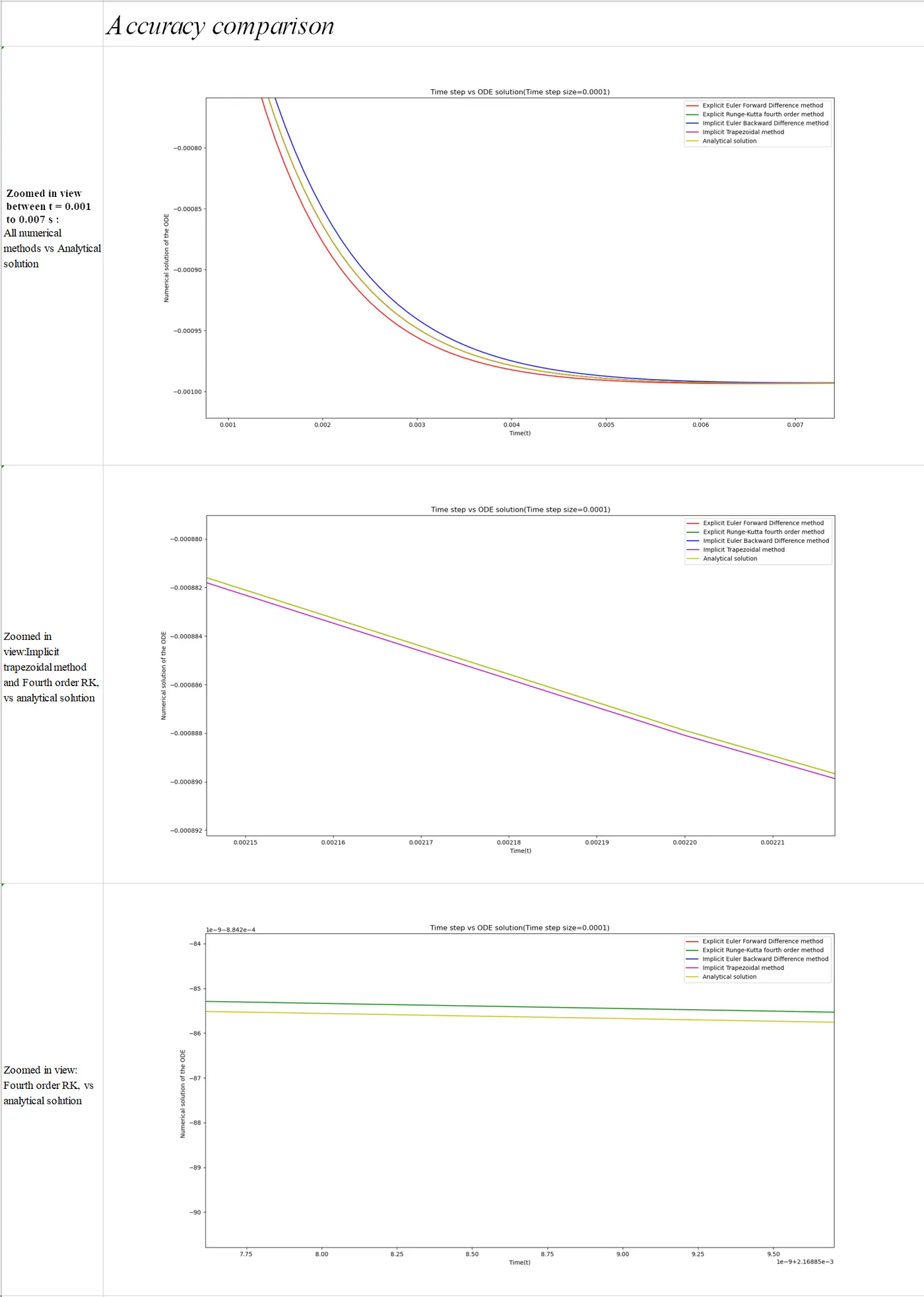
The following plot displays the accuracy of the solution(Time step size = 0.0001s).

Explanation:

Upon observation of the plots shown above, some superficial observations can be made.

• The forward difference method under-predicts the solution slightly, and the backward difference method over-predicts the solution. The error observed in both cases is obvious for this particular section of time, and can be attributed to the fact that both of these methods have an error margin of the first order, or rather, are first order methods. For such a small time step size, encountering stability issues is highly improbable, and the approximations can be relied upon.
• The implicit trapezoidal method has the second highest accuracy among all of the methods, and the margin of error is very small. This method has an error margin of the second order, since it is a second order method, and the accuracy of a second order method over the first order methods becomes obvious in this case.
• Finally, upon observing the plots and zooming in further, it can be seen that the explicit RK-4th order method has the highest accuracy, and is nearly indistinguishable from the analytical solution. The error margin is of the fourth order, and is the most accurate of the methods mentioned in this project.
• The accuracy of the implicit trapezoidal method and the explicit Runge-Kutta fourth order method are high, and for some of the plots, indistinguishable from the analytical solution.

Time step vs ODE solution:

Explanations:

1) Relationship between stability and time step size:

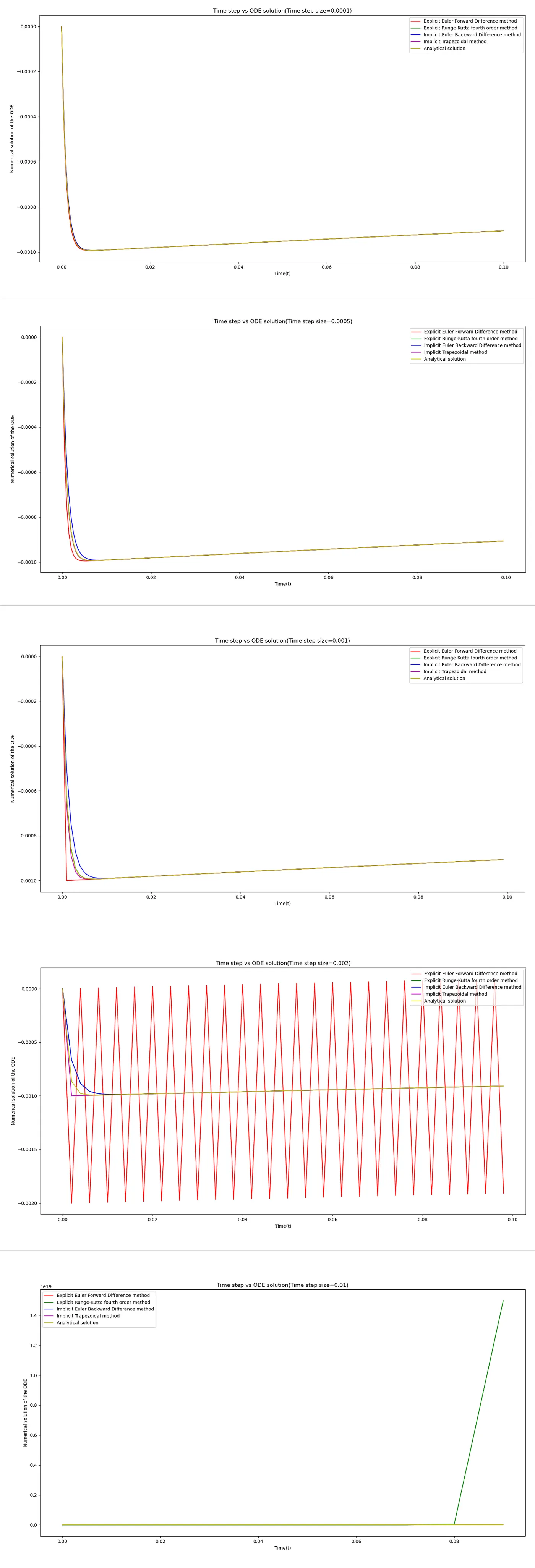
From the plots displayed above, it can be seen that there is a direct relationship between the stability of the numerical method and the time step size.

For a time step size of 0.0001 seconds, the approximations of the ODE solution are stable, with high accuracy.

Changes in accuracy are observed in the plot with a time step size of 0.0005 seconds. The implicit backward difference method and the explicit forward difference method start experiencing slight accuracy issues, as the numerical approximations begin to deviate away from the analytical solution. This behaviour is to be expected, as both methods are first order methods, as previously mentioned.

Peculiar changes in accuracy and stability are observed in the plot with a time step of 0.001 seconds. An unnaturally sharp edge is observed on the curve of the explicit forward difference method. This sharp edge is undesirable, but the solution is still within the stable range. This will be elaborated upon in the section about stability conditions. The other methods also begin experiencing the detrimental effects of a larger time step size, and can be seen in the curve for the implicit trapezoid method, that has begun deviating from the analytical solution, despite being a second order numerical method.

The numerical approximations of the ODE solution becomes unstable when using the explicit forward difference method, and the values provided by this method are unreliable,with a time step size of 0.002 seconds. The method fails to provide even remotely accurate values with the large time step size, and this may cause issues. The other methods begin to experience a drop in accuracy as well. But the implicit backward difference method manages to maintain stability and provides usable values, despite being of the same order. Even the implicit trapezoidal method begins to fail at this time step, and has an unnatural edge in its curve.

Hence, it can be concluded that step size has a direct effect on the solution stability, and a large step size may cause the ordinary differential equation to become unstable, for a particular numerical method.

The next segment will address the concept of stability in explicit and implicit methods.

2. Explicit methods:

Explanation:

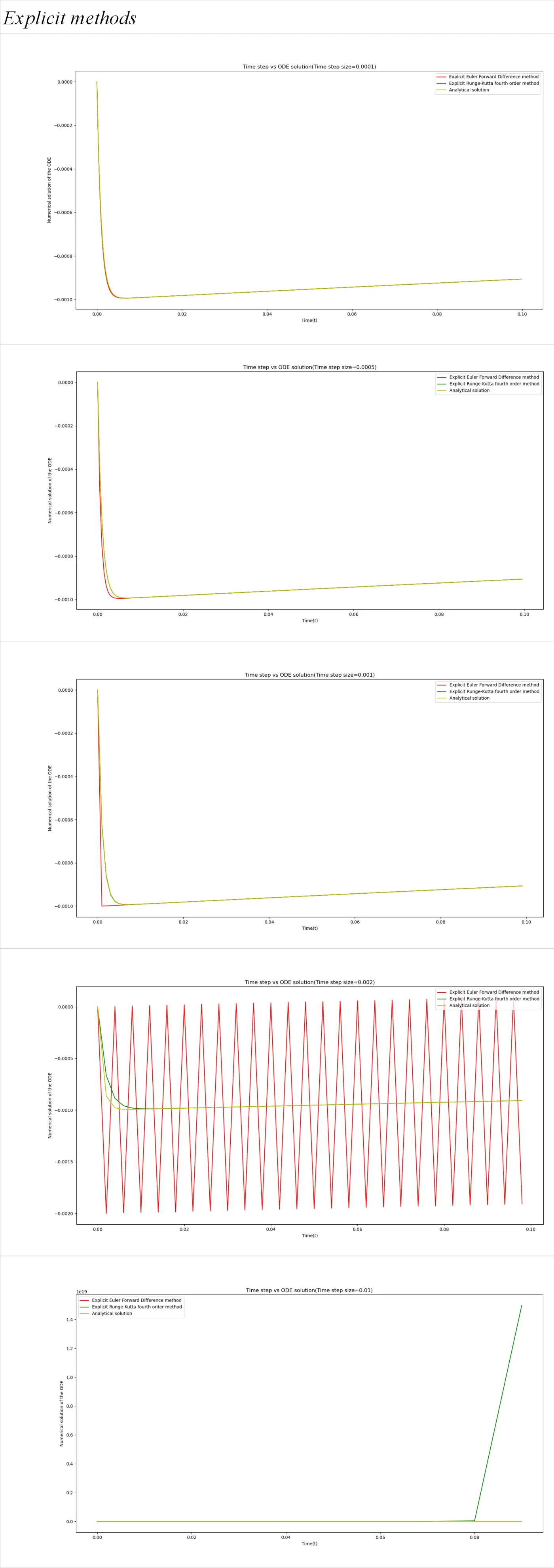
The behaviour of the forward difference method for the first three time step sizes have been elaborated upon in the previous section.

The Fourth-order Runge-Kutta method is markedly superior to the forward difference method in terms of accuracy and stability, for time step sizes of 0.0001s,0.0005s and 0.001s. The solution curve for this method is,for all intents and purposes, indistinguishable from the analytical solution with these time step sizes, and accomodates a larger time step more comfortably, compared to the forward difference method.

An interesting characteristic of the R-K fourth order method is it's capability to provide a stable solution at relatively a large time step, in this case, 0.002s. The forward difference method completely breaks down, while the R-K fourth order method still provides usable values, comparable to the implicit backward difference method mentioned in the first segment.

This may suggest that higher order explicit numerical methods have superior stability compared to lower order explicit(and some implicit numerical methods), for a certain range of step sizes.

Eventually the solution for the fourth order Runge-Kutta method becomes unstable and gives worse values compared to the forward difference method. However, this is a moot point, since the ODE solution for the forward difference method has already broken down and does not provide usable values, much before the ODE solution provided by the fourth order Runge-Kutta method begins to show instabilities.

3. Implicit methods:

Explanation:

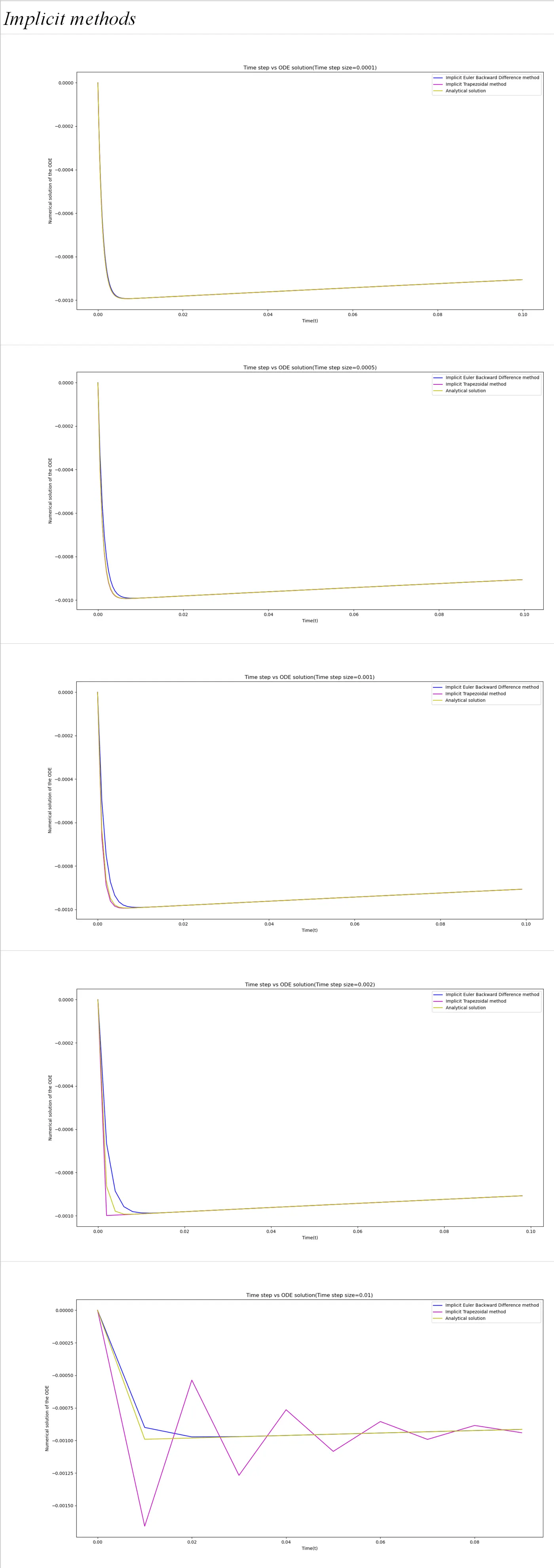
For the first three step sizes(0.0001,0.0005,0.001), the solutions provided by the numerical methods are as anticipated. The second-order Trapezoidal method has superior accuracy, compared to the first-order backward difference method. However, there are some interesting findings in the plots for time step sizes 0.002s and 0.01s.

As mentioned in the first segment, for step size 0.002, the solution stability of the Trapezoidal method seems to have been affected, due to the larger step size. But, the solution values provided first-order backward difference method seem to be unperturbed by this change, and give reasonably accurate and usable values.

Both of the methods are implicit methods, and the Trapezoidal method is of higher order. But despite this, the backward difference method provides more stable values, and this fact becomes even more apparent in the plot for step size 0.01.

The Trapezoidal method becomes unstable, and provides unusable values, but the backward difference method still provides reasonable values, and still manages to somewhat follow the trend of the analytical solution.

This phenomenon occurs, due to the difference in stability types. The Trapezoidal method is A-stable, while the backward difference method is L-stable. L-stability is a subset of A-stability. This difference is an important point, and will be explained in the next section.

Stability conditions, stability types and the effect of stability on engineering:

Each method has a stability condition associated with it, and the stability functions for each method(R-K 4th order not mentioned in this section) have been derived and mentioned below.

(i)Forward difference Euler method:

`y[i] = y[i-1] + dt*(f(t[i-1],y[i-1])`

`y[i] = y[i-1]-(1000*dt*y[i-1]) - (dt*e^(-1*t[i-1]))`

`y[i] =( y[i-1])*(1-1000*dt) - dt*e^(-1*t[i-1])`

Forward difference Euler stability function`= 1 - 1000*dt`

(ii)Backward difference Euler method:

`y[i] = y[i-1] + dt*(f(t[i],y[i])`

`y[i]= y[i-1] +dt*(1000*y[i] -e^(-t[i]))`

`y[i]= y[i-1] +(y[i]*1000*dt -dt*e^(-t[i]))`

`y[i]+y[i]*1000*dt = ((-dt*e^(-t[i])) + y[i-1])`

`y[i]*(1+1000*dt) = ((-dt*e^(-t[i])) + y[i-1])`

`y[i] = ((-dt*e^(-t[i])) + y[i-1])/(1+1000*dt)`

`y[i] = (y[i-1])*((1)/(1+1000*dt)) + ((-dt*e^(-t[i]))/(1+1000*dt))`

Backward difference Euler stability function `= (1/(1+1000*dt))`

(iii)Trapezoidal method:

`y[i] = y[i-1] + (dt/2)*(-(1000*y[i-1]) - e^(-1*t[i-1])-1000*y[i]- e^(-1*t[i]))`

`y[i]+((dt*500*y[i]+(dt/2)*e^(-1*t[i])) = y[i-1] -dt*500*y[i-1] - (dt/2)*e^(-1*t[i-1])`

`y[i]*(1+500*dt)+(dt/2)*e^(-1*t[i]) = y[i-1]*(1 -500*dt)- (dt/2)*e^(-1*t[i-1])`

`y[i] = y[i-1]*((1 -500*dt)/(1+500*dt)) - (((dt/2)*e^(-1*t[i-1])+(dt/2)*e^(-1*t[i])))/((1+500*dt))`

Trapezoidal method stability function `= (1-500*dt)/(1+500*dt)`

The variables associated with the numerical approximation of the solution at the current time step, forms the stability function of the method.

Hence, it can be said that stability conditions exist for all numerical methods, and help in evaluating the quality of the numerical approximation of the solution provided by a specific numerical method.

The use of stability conditions will be made evident in the following explanation regarding stability types.

Stability types and the effect of stability on engineering simulations:

The two stability types, A-stability and L-stability, will be discussed with reference to this project.

The following image displays the values of stability obtained after running the program, for each time step.

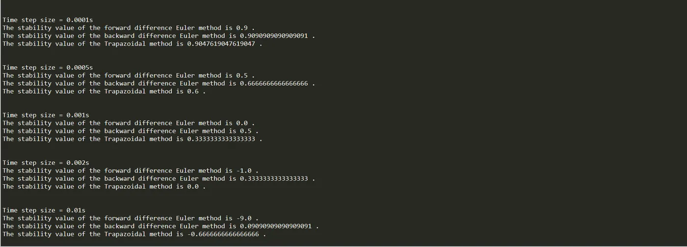
Upon observing the image above, the differences between stability types can be explained.

If the stability values of the Trapezoidal method are compared to the stability values of the Forward difference method, it can be seen that the values of the forward difference method tend to zero far more dramatically compared to the Trapezoidal method. The stability value crosses zero and becomes negative significantly faster, keeps decreasing, and seems to have no limit in the forward difference method.

The stability value of the Trapezoidal method however decreases at a much slower rate, but crosses zero eventually. However, it does not blow out of proportion and tends to a value of -1. The stability value of the Trapezoid method will never exceed -1, even with an unreasonably large step size value. But, this does not apply to the forward difference method. The forward difference method will give out unreasonably large stability values as the step size increases.

The behaviour exhibited by the Trapezoidal method is known as A-stability, and is generally a more favourable condition to have in a numerical method. The stability range of stability values that can be obtained is between -1 to 1, and if the stability value goes below 0, the solution becomes unstable.

A-stability does not apply to the forward difference Euler method, as the values obtained by the stability condition far exceed this range.

If the plot for the Trapezoidal method is observed, it can be seen that the plot for the numerical approximation of the solution does not blow out of proportion a large time step is considered, when compared to the forward difference method. In fact, it will never blow out of proportion, and will stay within a certain range, albeit inaccurate and undesirable. This is the advantage of an A-stable method, over a method that is not A-stable or L-stable, such as the forward difference method.

If the backward difference Euler method is observed, the stability values never dip below zero. In fact, it just tends to zero and never exceeds it and becomes negative. This type of stability is known as L-stability, which is a subset of A-stability. The stability range of an L-stable method is between 0 to 1. The speciality of this type of stability is the fact that the numerical approximations never blow out of proportion, and stay within range of the analytical solution, even with a large step value. The Trapezoidal method is not L-stable. This attribute has profound benefits in engineering simulations.

Stability of course, does not ensure accuracy, and a smaller time step should be used.

Stability is an important factor in an engineering simulation. As mentioned before, observing the stability of the ODE will provide an idea of how reliable the solution values are, for a given step size. Stability is greatly influenced by step size, and the step size must be chosen considering this factor. Different stability types exist for different numerical methods, and a specific method should be chosen keeping this in mind. Explicit solutions are faster, if not the fastest in terms of computational pace, but the solution are more likely to breakdown and become unstable if the time step is too large. In fact, explicit methods are the most sensitive to time step changes, and the accuracy of the solution provided by these methods is adversely affected due to this. Using a very small step size requires more computational time, and this can be undesirable for a problem with a large time period and does not require such extreme precision. Implicit methods may prove more useful in this regard, as they are A-stable methods, and ensure that the solution will not blow out of proportion. This is especially useful in problems with variable time steps. However, the computational time required by implicit methods are higher. But it compensates for this slight drawback by being able to accomodate a higher time step size while computing a solution while ensuring stability, and this is becomes an asset when the storage of computational data is considered. L-stable methods are the most stable, and never blow out of proportion if the time step is too large. These methods accomodate large step sizes comfortably, and is an important factor to consider in a simulation with variable step sizes.

Understanding the stability of a numerical method is imperative in choosing the optimal method, and in this way, has profound effects on an engineering simulation.

Google drive link for Python Code used and mentioned in this project: