Simulating fluid flow over the Ahmed body.

Aim : Simulating fluid flow over the Ahmed body, and observing the effects of its shape on the fluid by observing the wake region.

Introduction:

The Ahmed body and its importance:

A bluff body is a body that creates a separated flow region due to its geometry or shape, when a fluid flows over it. This characteristic is displayed by vehicles, as they are bodies that move at speeds high enough to cause this phenomena.

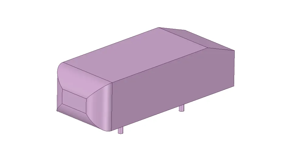
Fig.1.a : The Ahmed body

The Ahmed body is a bluff body that displays the effect of aerodynamic forces acting on it, a fair idea of the pressure, velocity and other variables, that would act on a vehicle under similar conditions. The Ahmed body may not look exactly like a vehicle, but it retains all its necessary basic aerodynamic characteristics, and is often used as a benchmark for simulating the fluid flow over a vehicle. Most importantly, the Ahmed body is utilized for its simple geometry.

The wake region past the vehicle is particularly of interest, as it displays the effect of the body on the fluid flow and the basic behaviour of aerodynamic forces. Since observing the behaviour of the fluid in the wake is of prime importance, the simple shape of the Ahmed body and its ability to display characteristics like drag, lift, pressure distribution, velocity and other effects, accurately, is an asset, as the geometry is simple to model and can save time by providing a fairly accurate estimate of the behaviour of said characteristics by subjecting it to different conditions, similar to real world conditions.

The angle of the rear inclination of the Ahmed body can be altered to observe the effects of the same, but is out of the scope of this project and will not be discussed.

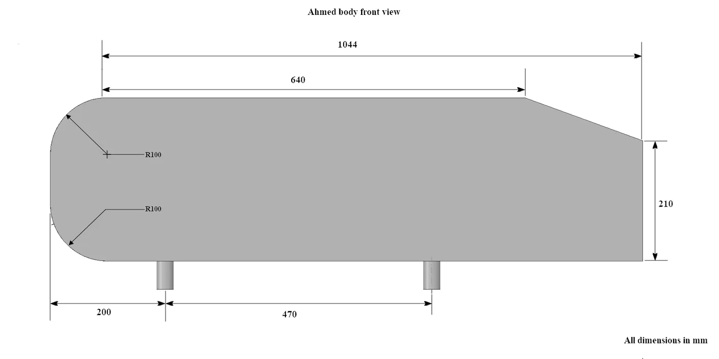
The following images show the dimensions of the Ahmed body.

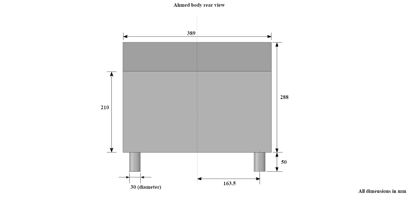Fig.1.b : The Ahmed body geometrical dimensions

Simulation process, modelling, mesh details and solver type used in Fluent :

The following steps were performed in order to simulate the fluid flow over the Ahmed body. The mesh details and solver type will be discussed within this section.

I) Geometry creation :

• The model geometry was created in SpaceClaim.
• Under the 'Prepare' option within SpaceClaim, upon creating the geometry, the 'enclosure' option was used to create three enclosures around the Ahmed body. The enclosures created contain the fluid domain that interacts with the Ahmed body.
• The enclosures progressively reduce in volume, growing closer to the Ahmed body, one inside the other. This has been done for mesh refinement purposes, the outer enclosure being the most coarse, while the smallest inner enclosure is meant to be much more fine. Three enclosures have been used in order to prevent a drastic drop in mesh quality, by refining the mesh in each enclosure somewhat gradually.
• The following image displays the location of this command and the dimensions of the enclosures.

Front view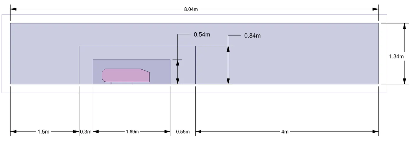
Side view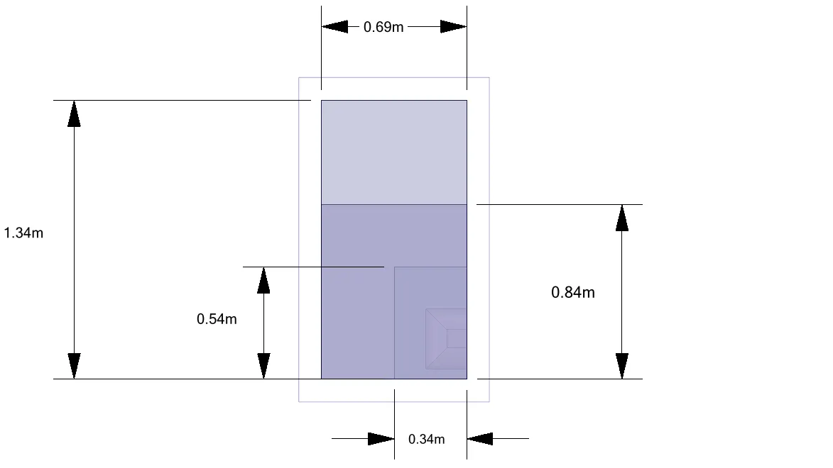

• There is a high chance of interference in the geometry after the creation of the enclosures, so an interference check was run to rectify any discrepencies in the geometry.
• The actual Ahmed body is suppressed for physics, as the forces acting within the Ahmed body are not required, and its basic shape is retained by the enclosures.
• Since the Ahmed body is symmetrical in nature, the geometry was split along its length through the middle, using the 'split body' command. The body was divided into two parts, and one part was removed, as the simulation time can be cut down while preserving the results.

II) Mesh creation and details :

After the creation of the geometry, the mesh was created by implementing a few techniques for obtaining an accurate result. The following are the techniques that have been used to create the mesh.

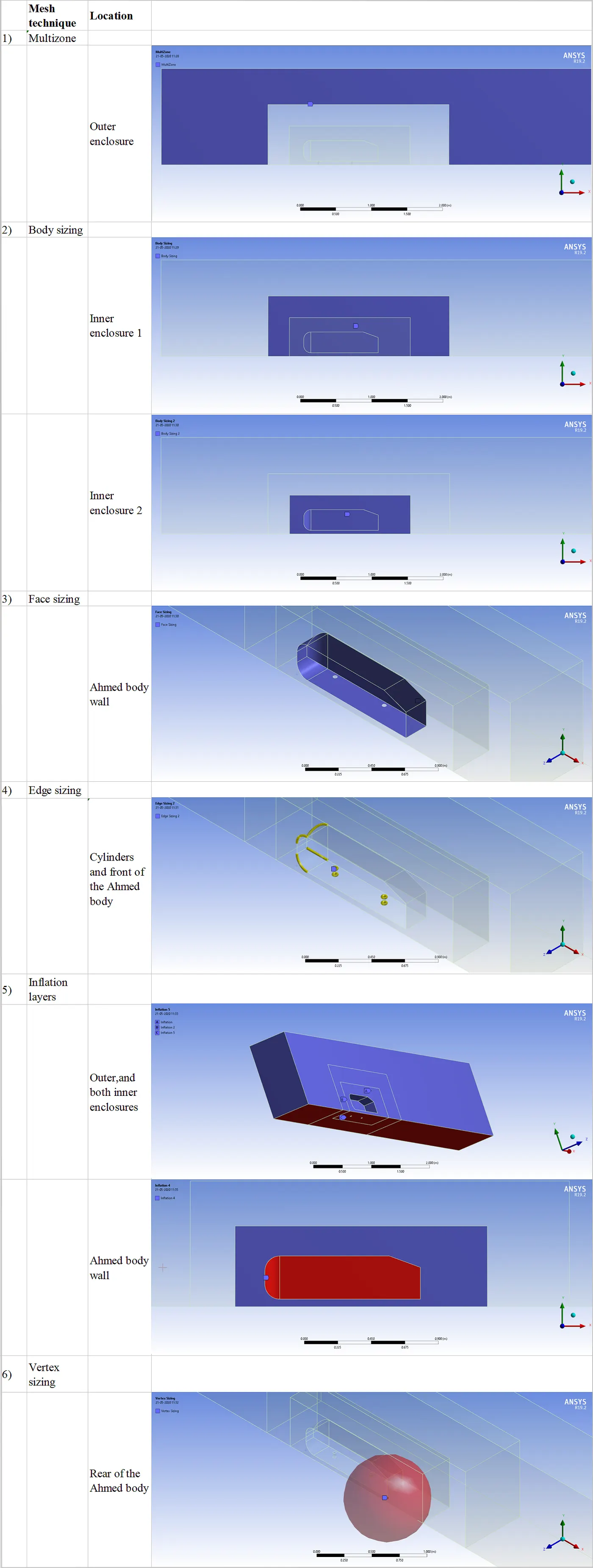
(i) Explanations:

1) Multizone :

• The multizone command is utilized to alter the default mesh type of the large enclosure to hexahedral mesh type. The advantage of performing this step lies in the computational time and direction of fluid flow. Utilizing a hexahedral mesh reduces the computational time, as it is a structured mesh, and structured mesh types yield better results for simple geometries, as the grid is aligned in the direction of flow.
• The flow development can be accurately computed, as the cells are more or less parallel to the wall. With the aid of the inflation layers (will be discussed below), the flow development of the fluid in the domain can be calculated accurately and at a relatively faster pace using the hexahedral mesh, compared to unstructured tets.
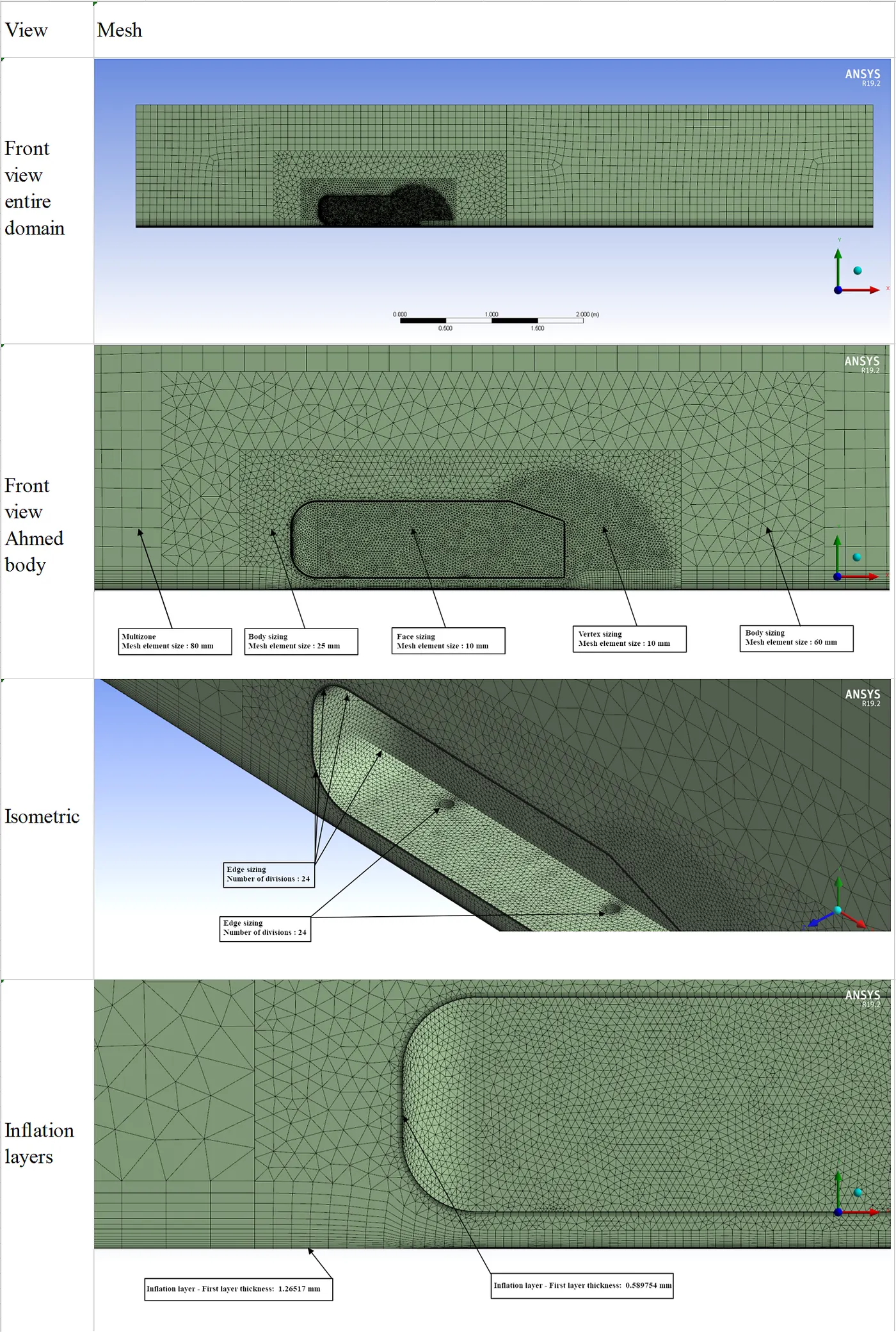
• The general element size in this domain is set at 80mm.

2) Body sizing :

• The body sizing command has been used on the two inner enclosures, in order to create a finer mesh around the Ahmed body wall. The smaller inner enclosure is the more refined, compared to the larger inner enclosure, in order to gradually increase the mesh quality as the Ahmed body is approached. This has been done in order to obtain more accurate results and to better capture the flow properties around the body, without using a fine mesh throughout the geometry, which would require higher computational time and would be unnecessary at locations without complex geometry.
• This enclosure contains a tetrahedral mesh, which is an unstructured mesh type, which is better suited for the relatively complex geometry of the Ahmed body (compared to the exterior enclosure).
• The element size set for the larger inner enclosure is 60mm and for the smaller inner enclosure is 25mm.

3) Face sizing :

• Face sizing has been performed on the Ahmed body wall in order to increase the accuracy of the computation of aerodynamic forces acting upon it, such as drag and lift. The pressure distribution over the Ahmed body walls can be accurately captured with a fine mesh, and hence, utilizing face sizing would prove to be advantageous in this respect.
• The face element size in this case is 10mm.

4) Edge sizing :

• The curvature of the front faces of the Ahmed body are important, as the angle of exit of the fluid flowing over it is dependent on it.
• Edge sizing has been used on the front face and the two cylinders below. This has been done in order to provide finer curvature to these particular surfaces, as they have a tendency to become polygonal in nature, after mesh creation. This happens if the mesh density is not enough to create a smooth curved surface.
• This step has been done by selecting these specific edges, and based on providing the number of divisions on the edge (shown in the image above) , a smooth curve can be obtained without increasing the density of the entire mesh.
• In this case, the number of divisions taken is 24.
• An important point to note is that the behaviour of this method should be set as 'hard', as this method can be overidden by other methods such as vertex sizing (will be discussed below) or face sizing, resulting in the same undesirable polygonal shape of the curve. This is especially important in the case of the cylinder near the rear of the Ahmed body, as it is in the sphere of influence of the vertex sizing method.

5) Inflation layers :

• Inflation layers are an important part of the mesh, as the fluid near the base wall, and the Ahmed body wall must be resolved accurately. Capturing the behaviour of the fluid near the wall is highly important, as it directly affects the results obtained by the simulation. The inclusion of the inflation layers has been done to overcome computational inaccuracies, as the mesh element size is not fine enough to capture near-wall fluid behaviour.
• The size of the first boundary layer has been set by calculating its size by using the value obtained at a suitable Y-plus value. Using the correct Y-plus value is an important part of this step, as the ideal thickness of the first layer near the wall determines the accuracy of values such as lift and drag.
• This also depends on the solver being used and the nature of the flow. For this simulation, a k-omega SST solver will be utilized and will be discussed in a section below.
• A Y-plus value of 20 has been chosen for this particular case, as the recommended value for Y-plus for a k-omega SST model is above 11.
• For the inflation layers at the bottom,the entire body is selected, and the layers grow from the base wall of the domain. For the inflation layers around the Ahmed body, the body is selected as the boundary, and the layers are stacked over the Ahmed body.
• A growth rate of 1.2 is set, so the cell size grows as we proceed to move away from the wall.
• The calculated height of the first layer above the Ahmed body wall is 0.589754 mm, and for the base wall, is 1.26517mm.

6) Vertex sizing:

• In order to obtain the most accurate behaviour possible of the fluid in the separated region, the region where flow separation occurs is highly refined by utilizing the vertex sizing method. A point at the end of the rear of the Ahmed body is used as the vertex center, and a sphere of influence of radius 0.4 m has been created. The sphere covers the entire rear section of the Ahmed body, and the volume within which flow separation occurs.
• The element size within to sphere of influence is set to 10mm.

The following images display the final mesh created by using the techniques mentioned above.

(ii)Named selections:

The following images display the named selections of the geometry.

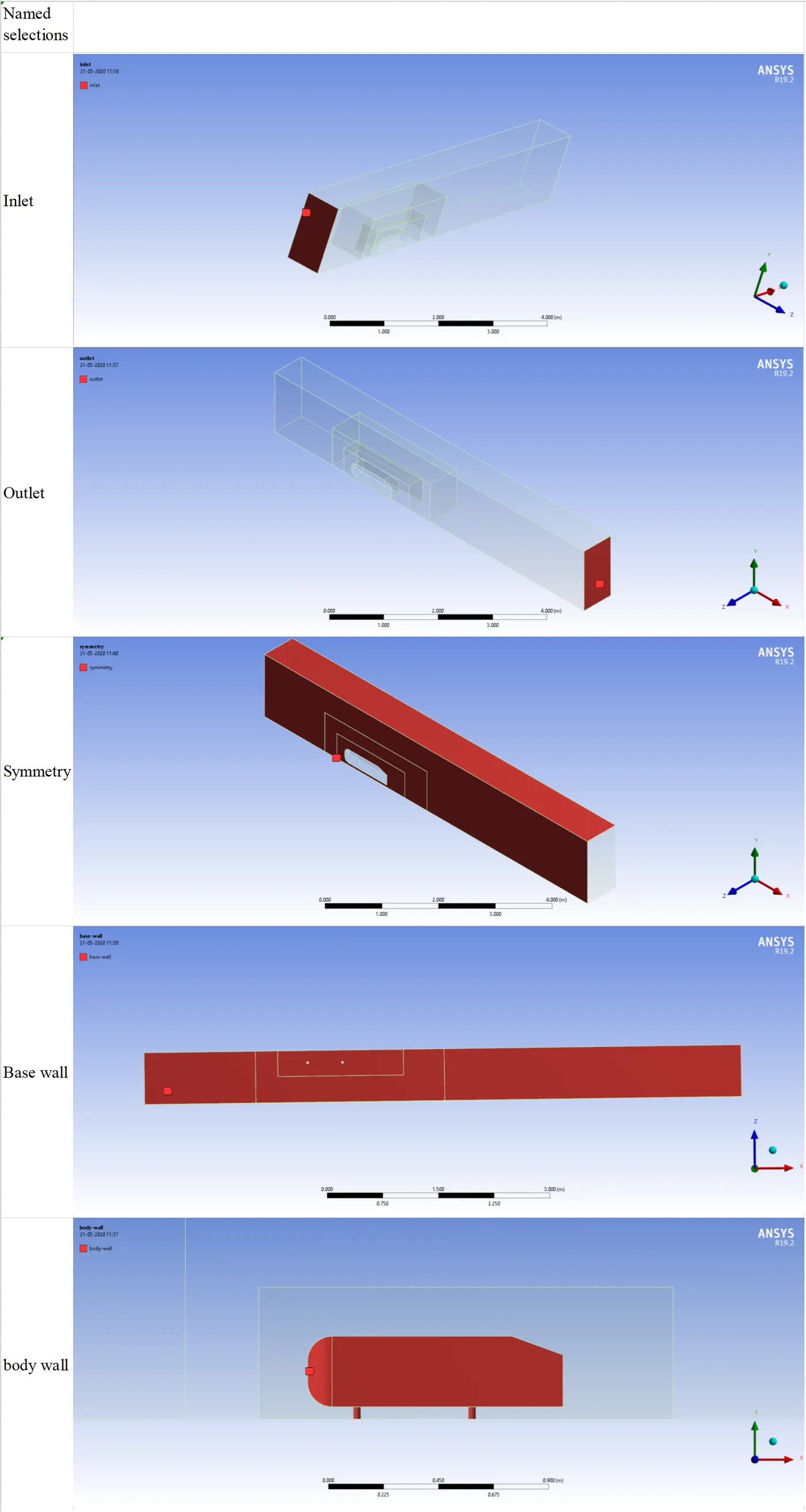
• The named selections are created by selecting the required face and naming that particular face.

III) Model details and Fluent set up:

(i) Model used :

• k-omega SST

Explanation :

• The k-omega SST turbulence model has been selected for this simulation due to the fact that it provides accurate simulation results for separated flows due to blunt bodies. The k-omega SST model has been designed to contain the benefits of both, the k-epsilon and k-omega models. The k-omega model solves the near-wall functions accurately, but is inaccurate in the freestream velocity sections of the fluid flow, whereas the k-epsilon model accurately solves the freestream section of the fluid flow, but provides inaccurate values at the near wall or viscous sub-layer section.
• The k-omega SST model uses a k-epsilon model in the freestream sections of the fluid flow, and a k-omega model for near-wall computations.
• This seamless switching between models is done by the integration of two blending functions 'F1' and 'F2'.
• If the value of F1 is zero, the model switches to the k-epsilon model. Similarly, if the value of F1 is one, the k-omega model is used.
• F2 involves the use of a viscosity limiter, which prevents the model from over-predicting the wall shear stress, and functions similar to F1.
• Due to the nature of the flow, the recommended Y-plus value is above 11.

(ii) Solver type:

• Density-based

The density- based solver has been used to capture the effects of compressibility, since the body is a bluff body and flow separation takes place. A pressure-based solver can be used as well, but the accuracy of a density-based solver is slightly higher when it comes to such flows.

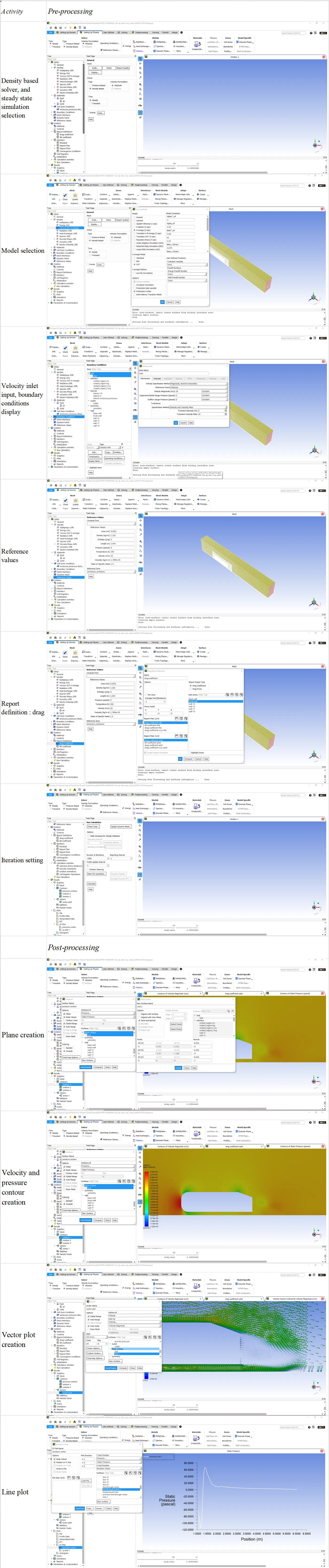
(iii) Fluent set-up :

Pre-processing:

• After the mesh is imported into fluent, the solver type is changed to Steady State, Density based, under Setup > General, in order to account for any compressibility effects, due to the nature of the fluid flow.
• The model is changed to k-omega SST under Setup> Models > Viscous, for the reasons mentioned in the previous section.
• The freestream velocity is set to 25 m/s, from the inlet, by going into Setup > Boundary Conditions > Inlet. This will be displayed in the table below. The boundary conditions of the simulation are under the same section under 'Type', and can be changed by using the dropdown provided below in the section.
• The boundary conditions are set in Fluent, as shown in the table below.

NAMED SELECTION	BOUNDARY CONDITION
Inlet	Velocity inlet
Outlet	Pressure Outlet
Symmetry	symmetry
body wall	wall
base wall	wall

• The reference values for lift and drag are provided by entering Setup > Reference values, where the area of half of the Ahmed body (A = 0.0551 m) is entered, since the simulation is being run by considering only half of the Ahmed body. The area considered is across the Ahmed body, perpendicular to the direction of flow. The velocity is set as 25 m/s, keeping the other variables the same, as the working fluid is air, which is assumed by default.
• The plots for lift coefficient and drag coefficient are created by going into Solution > Report definitions, and selecting the Ahmed body, since we require the lift and drag coefficient values over that surface.
• The number of iterations is set to 1600 by going into Run calculation, and hence, running the simulation.

Post-processing:

• The pressure and velocity contours are obtained by going into Results > Graphics > Contours.
• The velocity vectors are obtained by entering Results > Graphics > Vectors.
• The line plot shown in the Result section has been obtained by going into Results> Plots > XY plot. Within this section, a line that passes through the vortex (discussed in the next section) is created, and subsequently, the pressure over the lines length is plotted and displayed in the Result section.

The image below displays all of the set-up related sections mentioned above.

2) Presence of negative pressure in the wake :

• If the static pressure of the section along the length of the domain is shown on a contour, a peculiar result is observed. Negative pressures are seen in the wake, if static pressure is shown on the contour plot.
• This does not suggest the existence of actual negative pressure, as Fluent displays the gauge pressure of the fluid, not the absolute pressure. By definition, the gauge pressure is dependent on the atmospheric pressure, and basically displays pressure based upon this, using atmospheric pressure as a benchmark.
• The negative pressure values that have been obtained in that region simply indicate that the pressure in the wake is below atmospheric pressure (101325 Pa).
• To put it simply, the pressure in the wake region is simply below atmospheric pressure, and the reason for this pressure drop will be explained in the next section.

3)Results:

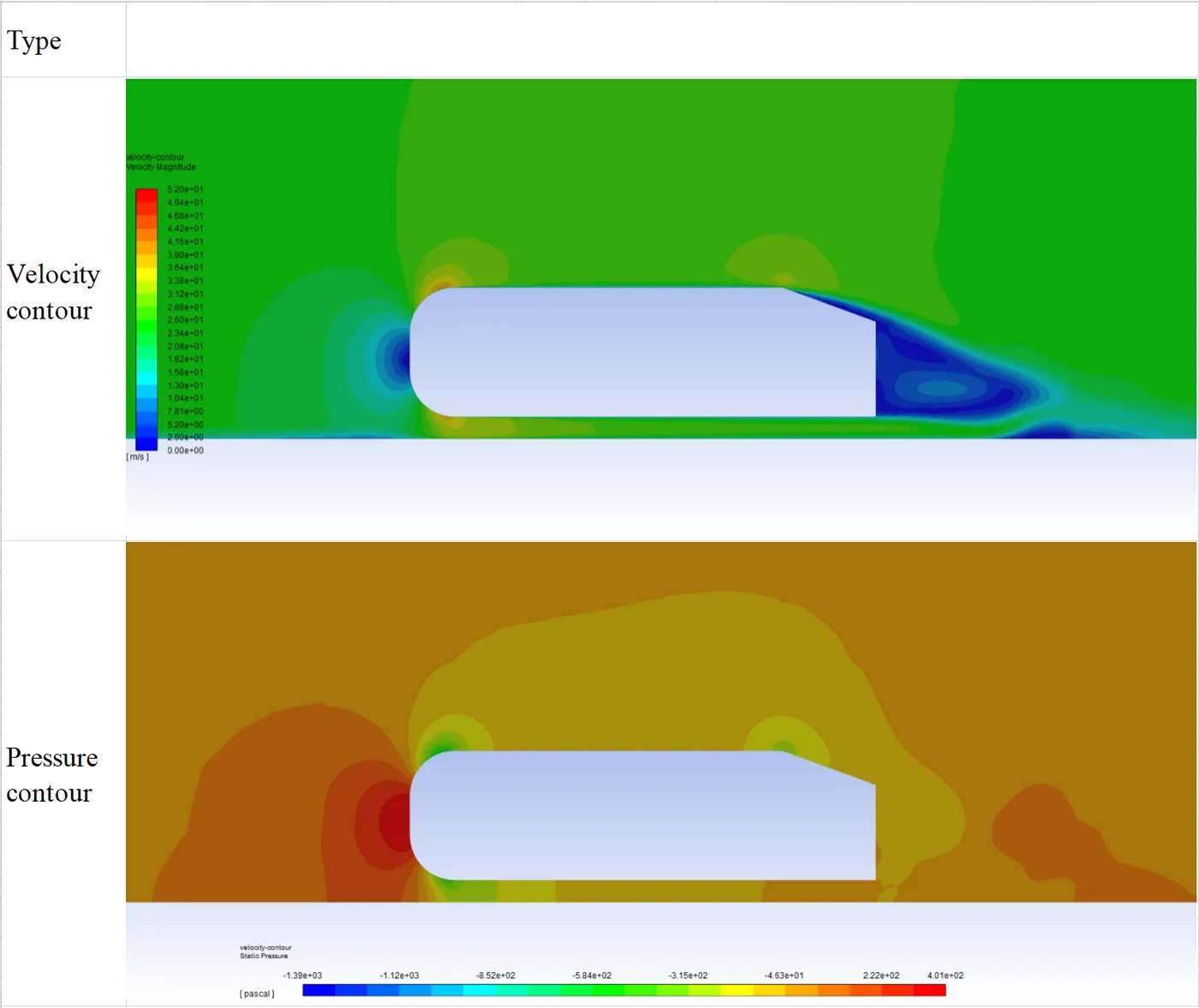
• The following image displays the velocity and pressure contours of the area around the Ahmed body:

a) Low pressure region behind the Ahmed body, point of separation and flow separation :

• If the contour plot for pressure above is observed, the pressure acting on the front of the Ahmed body is high, and the pressure around the curvature of the front is much lower in comparison. The increased pressure of the fluid in that region affects the fluid surrounding it, the velocity of the fluid in particular. The increased pressure in that region applies a force on the fluid in the direction of flow, and the velocity of the fluid increases as it flows over the curvature of the front face of the Ahmed body. Since the velocity of the fluid over the bend has increased, the pressure in that region decreases. This suggests that the forces acting on the fluid are in the direction of flow, and for the sake of explanation, it can be said that the high pressure at the middle front face pushes the fluid over the bend, and the low pressure on the curvature pulls the fluid over the bend. This phenomenon is known as favourable or negative pressure gradient, the static pressure decreases in the direction of the flow.
• However, at the rear of the Ahmed body, the fluid behaviour changes. At the top of the inclination of the rear face of the Ahmed body, a pressure drop is observed, and this can be attributed to the increased velocity in that specific region. The velocity increases due to the sudden inclination, as the frictional forces at that distance drop significantly due to the absence of the wall. This increase in velocity causes a pressure drop in that region. This is an important point to note, as it plays a role in the formation of the point of separation.
• If the rear part of the body is observed carefully, the fluid flow separation begins near the top of the inclination of the rear part of the Ahmed body. The velocity of the fluid is high at the top of the inclination, and the fluid seems to 'jump' over the inclination, instead of flow over it. But the velocity of the boundary layer reduces significantly, and the pressure near the top of the inclination has dropped. This suggests that the sudden incline has caused a reduction in kinetic energy in the boundary layer, which can be seen in the vector plot. In the pressure contour plot, it can be observed that the static pressure along the inclination is increasing. The kinetic energy or velocity of the boundary layer must be more than a certain limit in order to overcome the pressure opposition in the direction of flow, if it is to remain attached to the inclination. But, the energy possessed by the boundary layer is insufficient due to the low pressure region near the top of the inclined rear wall of the Ahmed body, and the velocity is not enough for the boundary layer to continue flowing over the inclined rear wall of the Ahmed body, causing it to separate from the surface.
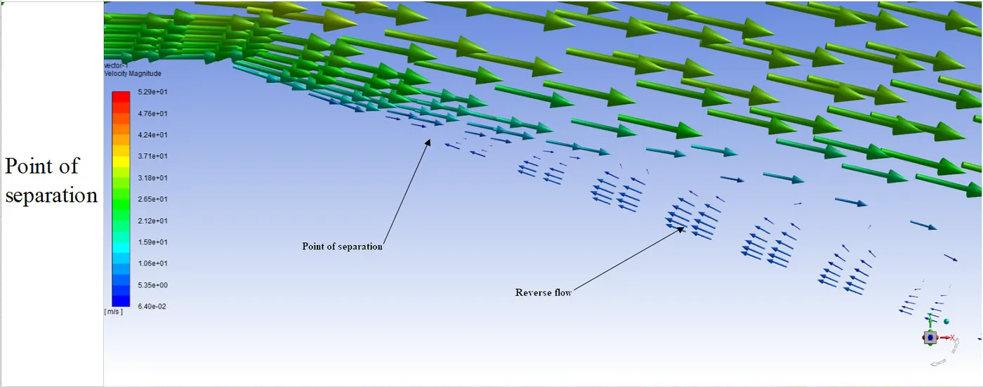
• This behaviour is caused by a phenomenon known as adverse pressure gradient. This occurs when the fluid flows from a low pressure region into a high pressure region. The point at which this phenomenon occurs is known as the point of separation. The velocity near the wall is almost zero (excluding the no-slip condition).
• An important point to note is that the formation of the flow separated region behind the Ahmed body is a consequence of this phenomenon.
• As the boundary layer separates from the inclined rear wall of the Ahmed body at the point of separation, a region of fluid with low pressure and low velocity is formed, and is known as a flow separated region. This region exists for a certain length and volume within the wake, and ends at a point known as the re-attachment point. The re-attachment point is established when the velocities of the separated fluid flow streams (in this case, the fluid flowing under the Ahmed body and the fluid outside the flow separated region) attain similar values and meet again at a point ahead in the fluid domain, creating a closed volume of fluid.
• The fluid outside the flow separated region possesses much higher kinetic energy, compared to the kinetic energy possessed by the fluid within the flow separated region, hence preventing the fluid within it from leaving the enclosed volume. This leads to the formation of a low pressure and low velocity region behind the Ahmed body. This can be seen in the velocity contour plot shown above.
• The low pressure of the flow separated region affects the fluid flowing just outside this region, as it exerts an inward pulling force on the liquid outside the flow separated region. This force is sufficient enough to draw some of the fluid at the boundary of the flow separated region, within its volume, hence reducing the velocity of this fluid. But since the fluid possesses inertia, it follows a curved flow path, instead of directly entering the flow separated region.
• It is due to this behaviour, formation of vortices within the flow separated region can be observed.
• The following images displays the vector plots for the region surrounding Ahmed body (vector plots scaled to 20, 10 and 20 respectively)

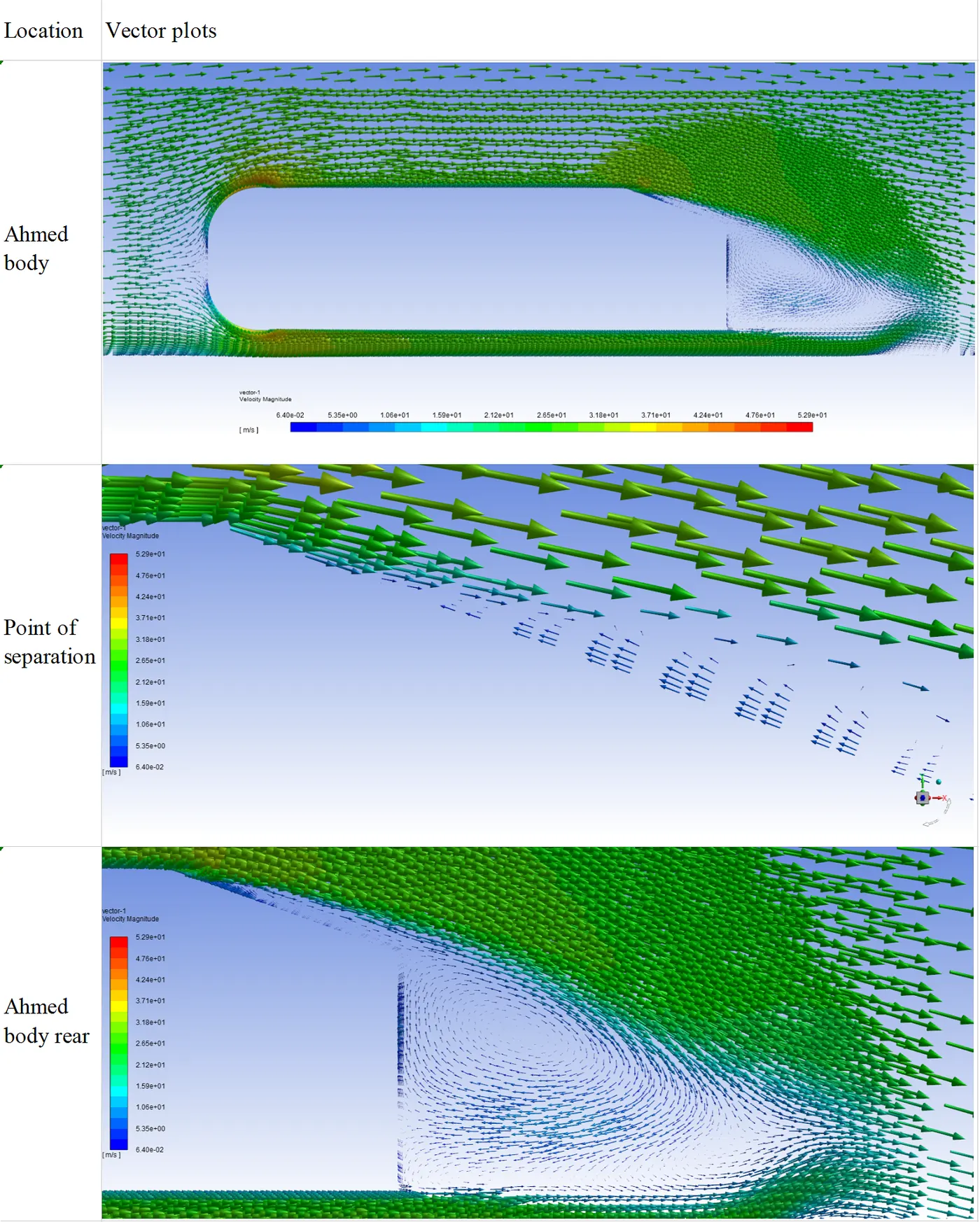
• The formation of a vortex causes fluid backflow, as the vortex appears to rotate in a counterclockwise direction, and possesses some energy at this point. The backflow occupies the region post separation point.
• A point to note is that like flow separation, the backflow is a consequence of the formation of the point of separation, and not vice versa.

Drag and lift coefficient:

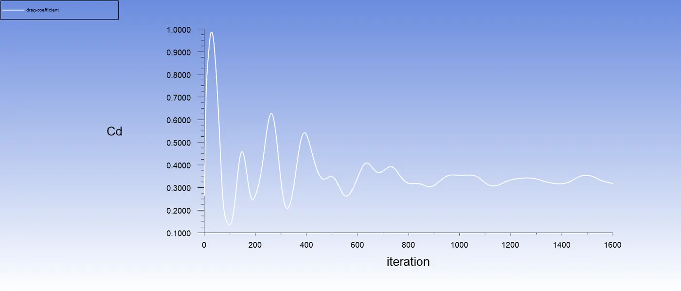
The following image displays a drag coefficient plot over 1600 iterations.

Drag coefficient:

Lift coefficient:

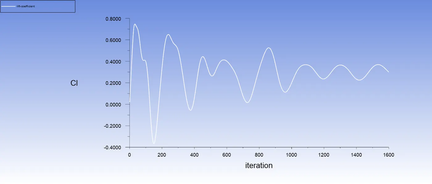
• From the above plots, a drag coefficient of 0.31530319 and a lift coefficient of 0.29148196 has been obtained after running the simulation for 1600 iterations.
• The lift and drag coefficient are affected by the formation of vortices in the rear of the Ahmed body, and are the cause of the oscillatory behaviour in the plots shown above.
• Another important point to note is that the drag acting on the body is pressure drag, caused by the recirculation or flow separated region at the rear of the Ahmed body, as the vortices increase drag on the body.

Grid dependency test:

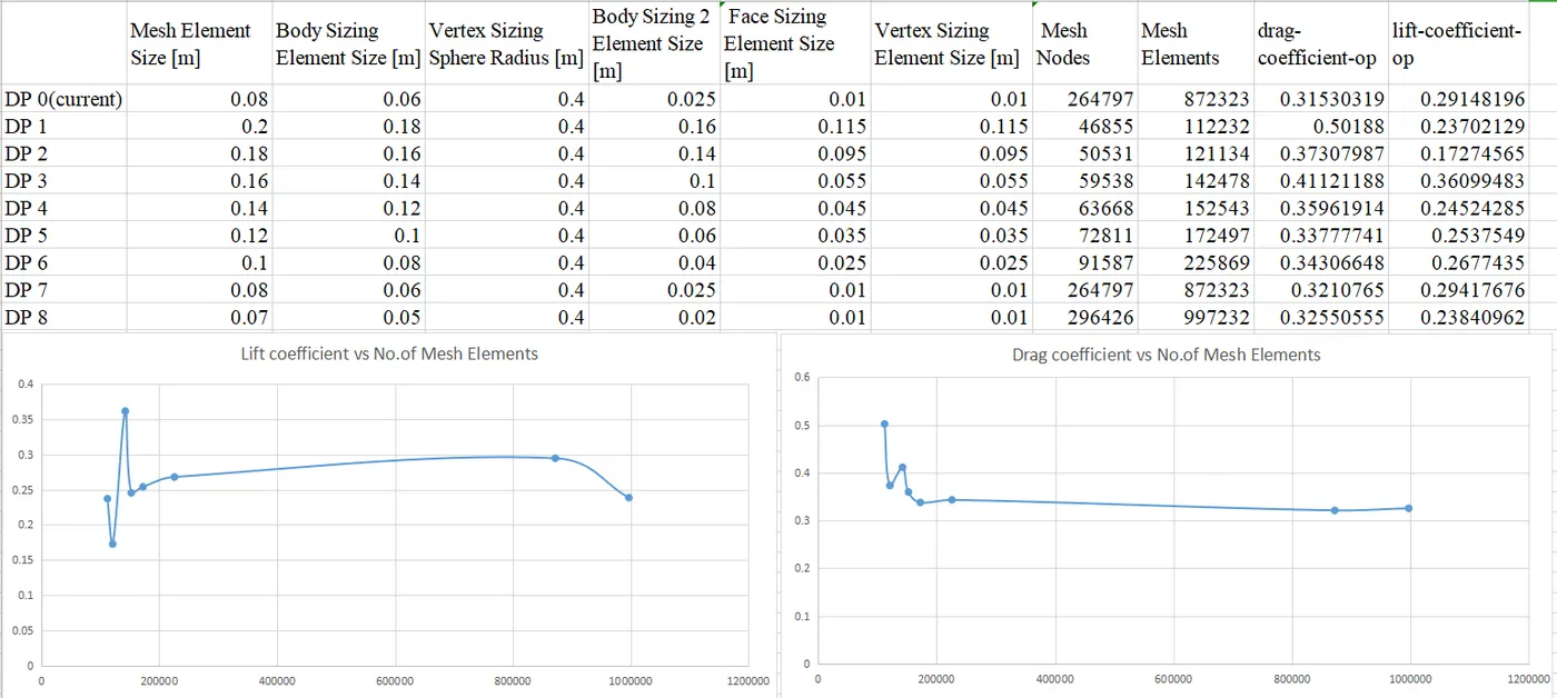
The grid dependency test was performed using the parametric analysis method.

This method takes into consideration a few factors that contribute to the mesh creation, and are varied in the parameter set section.

Parameters varied:

• Mesh element sizes of all three enclosures, defined by Body Sizing.
• Mesh element sizes of Ahmed body faces, defined by Face Sizing.
• Mesh element size of the sphere, defined by Vertex Sizing.

All of these parameters have been varied as mentioned in the 'Mesh creation and details' section above. The differences in element sizes of each component have been maintained for all the cases.

Variables observed:

• Lift coefficient
• Drag coefficient

The effect of changing the mesh element sizes of different parameters are observed, using the drag and lift coefficients(in this particular case). The mesh density plays an important role in this test, as after a certain point of mesh refinement, changes in the variables(drag and lift coefficients) will not be seen. At this point , the mesh configuration of the second highest number of mesh elements can be selected.

Performing this test is important as the results obtained are affected by mesh density, and a mesh that is too coarse will provide inaccurate results. Also, using a mesh that is more refined than what is required will only result in an unnecessary increase in computational time.

Steps:

• Parameters are selected in the 'Meshing' section, and are automatically imported to the Parameter set. A small box next to the parameter is to be selected(will be highlighted with a blue background with a white 'P' in the middle) in order to transfer the parameter into the Parameter Set.
• Variables are selected in the 'Fluent' section, namely, Drag and Lift coefficient, using the Create Output Parameter option.
• The simulation is run, with the required settings. While exiting, an option for 'Use settings for current and future calculations' will appear, and is selected. If this step is not performed, the results obtained by Parametric analysis will be incorrect, as it will not use the values entered in the 'Report definitions' section.
• The Design Points are created, and the values of the parameters mentioned above are varied, causing a change in mesh density, and will be seen under the 'Mesh Elements' section.
• The Design Points are updated and the lift and drag coefficients are obtained.
• The table is imported to Excel, where plots of 'drag coefficient vs mesh elements' and 'lift coefficient vs mesh elements' are created.
• Upon observing the graphs, the suitable mesh configuration is selected for running the actual simulation.

Parameter selection in Meshing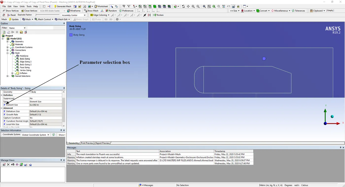
Variable selection in Fluent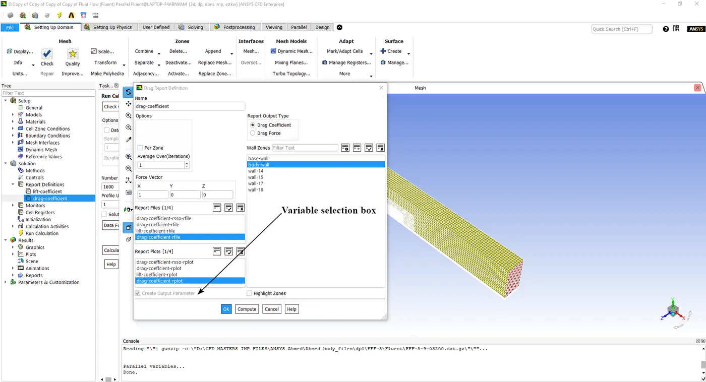
Parameter set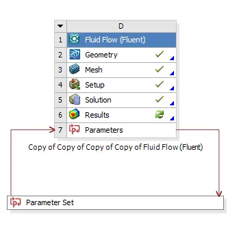
Parameter set display(Design points)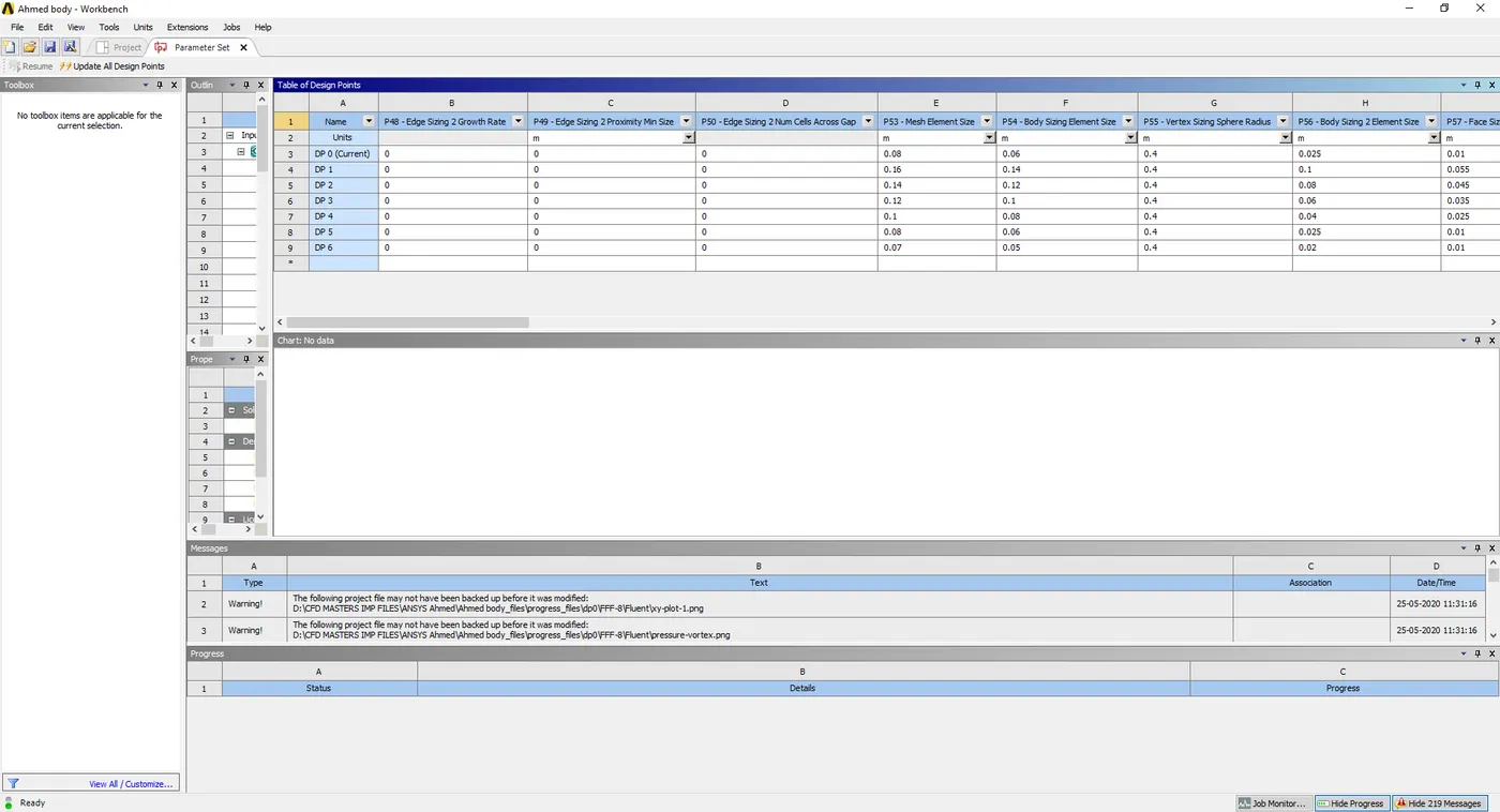
Parameter set display(Variables)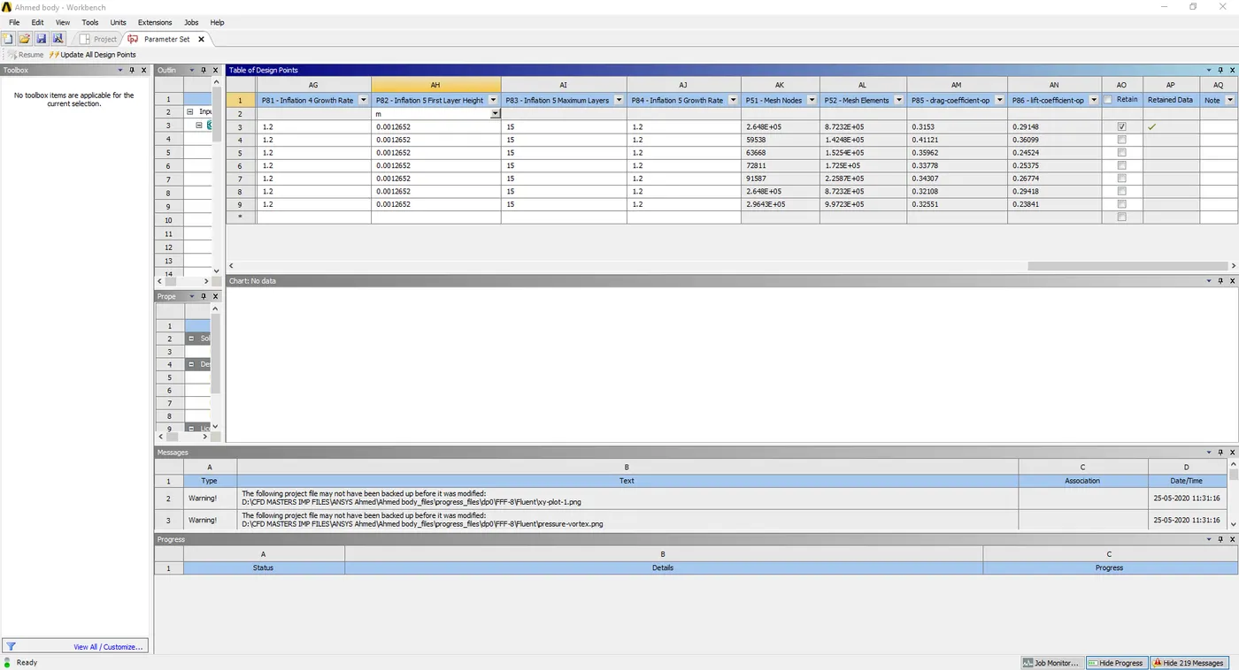
Excel table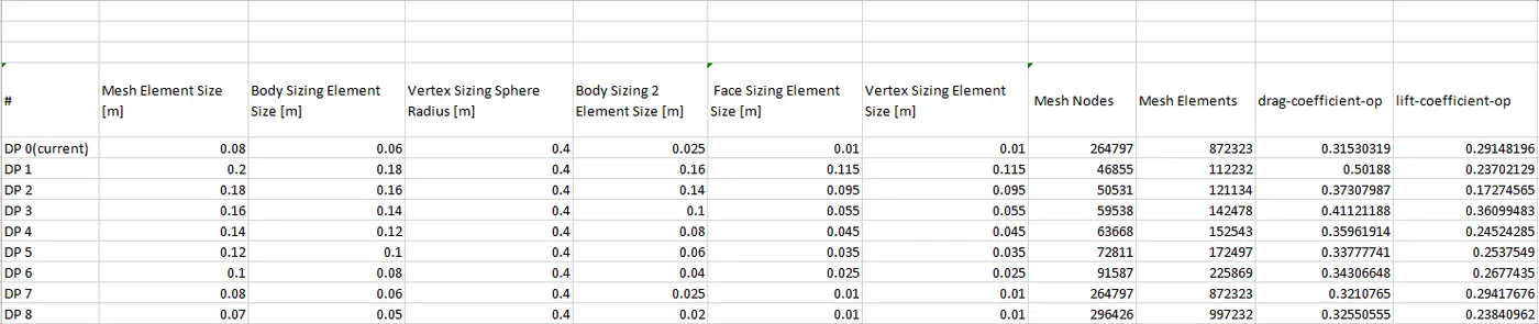

Parametric analysis results:

Upon observing the lift coefficient vs no.of mesh elements graph, the ideal mesh configuration cannot be seen as the results are varied and do not show a definitive pattern. Hence the plot for lift coefficient vs no.of mesh elements will be taken into consideration.

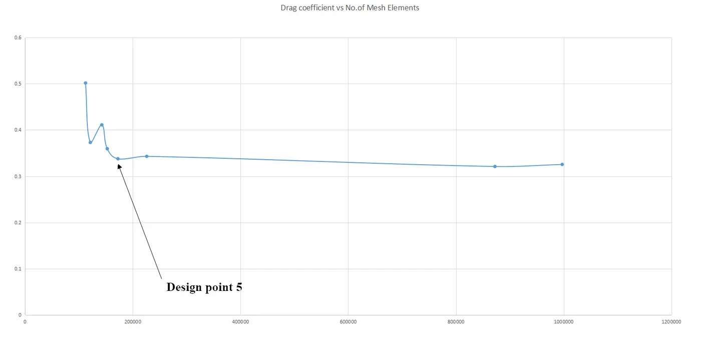
Drag coefficient vs no.of Mesh Elements:

• Upon observing the graph, the ideal design point appears to be design point 5, with Mesh Element count of 172497.
• The variation in the drag coefficient seem negligible, and this configuration can be selected for sufficiently accurate results.
• For this particular simulation however, design point 7 has been selected in order to observe the behaviour of velocity vectors in the flow separated region in more detail.

Conclusion:

The behaviour of the fluid in the wake, and the formation of the vortices in the recirculation or flow separated region has been observed in great detail in this project. An important finding of this simulation is the formation of the flow separated zone, which is a consequence of boundary layer separation at the rear inclination of the Ahmed body. The understanding of favourable and adverse pressure gradients in this project was imperative for understanding the behaviour of the fluid over the Ahmed body, as adverse pressure gradient is the cause of the boundary layer separation. Both phenomena were observed over the geometry of the Ahmed body, and it can be concluded that both velocity and the geometry of the Ahmed body play a vital role in the formation of the flow separated region. The inclination of the rear face of the Ahmed body would most definitely affect the position of the point of separation, and will have an effect on the drag and lift over the Ahmed body.

Another learning of this project is the importance of choosing the ideal model for simulation of separated flows, as different models have different advantages and disadvantages, and selecting the ideal model is imperative in obtaining an accurate simulation of the flow over the body. Selecting the Y-plus value and number of inflation layers over the body was another important lesson that was obtained during the duration of this project.