Week 5 - Rayleigh Taylor Instability

Aim : To simulate the Rayleigh-Taylor instability using water and air for different mesh element sizes, and a user-defined fluid with water.

Introduction:

The Rayleigh-Taylor instability is a phenomenon that occurs at the interface of two fluids of different densities, with the denser fluid on top of the less dense fluid. The difference in the potential energies possessed by the two interacting fluids causes an instability at the interface of the two fluids. Fluids of different densities exhibit different instability behaviour, and this is will be elaborated upon in detail in this project. Various mathematical models have been tailored to solve the Rayleigh-Taylor instability.

Mathematical models that capture the physics of this phenomenon are the Potential Flow model, Incompressible flow model, Isobaric flow model and the Viscous Flow model. Each of these models have their own assumptions about the divergence and curl of the vector field, and assumptions about the density of the fluid. Some form of these models and their assumptions are used in CFD, and some CFD models that can solve the instability at the interface are the Volume of Fluid model, K-L turbulence model, and Diffuse Approximated Method. These models solve the governing equations of momentum, volume fraction and other equations using numerical approximation schemes that are implicit or explicit in nature. These schemes offer their own benefits in terms of stability, accuracy and computational time. These models use methods such as the Finite Element Method in order to discretize and solve the non-linear governing equations of the fluid phases in the domain, and this will be observed in this project.

Simulation workflow:

Solving and Modelling approach:

• For this simulation, a two fluids of different densities are required. Water and air was used for the first part of this simulation, and a user-defined fluid with a specified density and viscosity was used for the second part of this simulation.
• The simulation performed was two-dimensional in nature, as it is computationally less expensive and will accurately capture the behaviour of the fluids at the boundaries.
• A conformal quadrilateral mesh can be used, as the two-dimensional geometry is a simple two-dimensional rectangle. Using a quadrilateral mesh element type is preferred, as the accuracy of the results obtained are higher compared to a triangular mesh, as the mesh skewness value is kept under control with a quad mesh element type.
• The mesh element sizes that were used in this simulation were 0.5mm, 0.2mm and 0.1mm. The effect of mesh density will be elaborated upon in the Results section.
• The simulation type was transient in nature, and benefits of using a transient simulation over a steady-state simulation will be explained in the Results section. The general behaviour of the fluid under these conditions are known to us, and the end state of the simulation is already known to us. A transient simulation will allow us to investigate the behaviour of the fluid at particular points of time, before it reaches steady-state, and this is the objective of this project.
• Since two fluids are involved in this simulation, the Volume of Fluid model will be used, as it has the capability of calculating the volume fraction of the fluids interacting in the domain over a period of time. The solver-type used will be pressure based for this case, as the pressure field is what couples the two interacting phases. This is important, as the pressure field also couples the momentum equations that will be solved. The momentum equations will be solved for both the phases.
• An important attribute of the VOF model is that a cell volume can only contain of the two phases that have been considered. This means that the volume fraction of a fluid phase in a cell can be either 0 or 1. To put this in context, the cell volume can contain either water or air, but not both(in this case).
• The implicit protocol of obtaining the volume fraction will be used, as the stability of the solution will be higher, and less sensitive to the time step size.
• The Viscous model has been specified as laminar, and will solve the Navier-Stokes equations for the flow in the domain.

I) Geometry creation:

• The geometry was created using SpaceClaim.
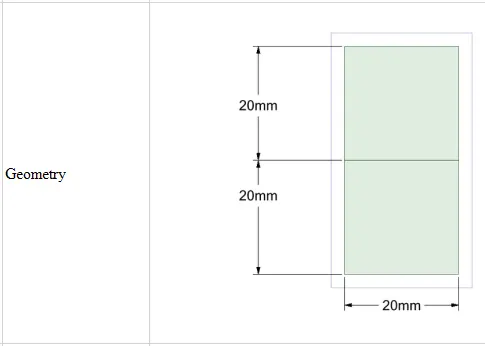
• In order to create the two fluid phases that will be interacting with each other, two square shaped geometries were created. The 'Pull' tool was used in order to create the two 2-D surfaces(Design > Pull).
• The two geometries are meant to share an edge, and this was done by using the 'Share' tool(Workbench > Share).
• This will allow us to create the interface at which the two fluids will interact.

II) Mesh creation:

• The geometry was imported into the meshing module.
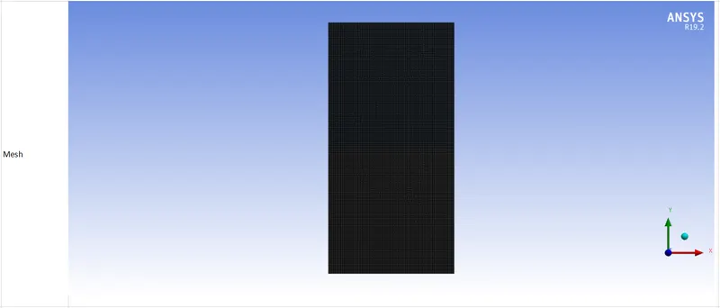
• The element size was specified as 0.5 mm(0.2mm and 0.1mm for the other cases), and quadrilateral conformal mesh was created. This type of mesh will yield highly accurate results, as the mesh skewness value is kept low and under control.

III) Fluent settings:

(a) General settings:

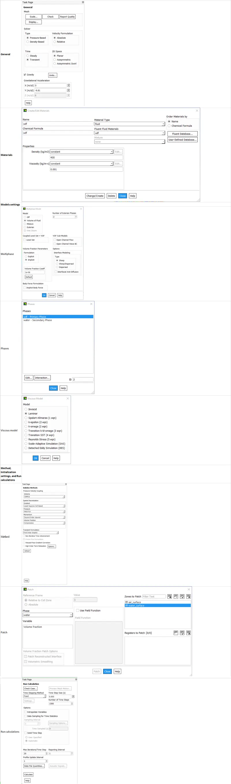
• The simulations that are going to be carried out are steady state in nature. This is set in the General section(Setup > General). Acceleration due to gravity is switched on as well, and a value of -9.81 `m/s^2` is given, with the negative sign indicating the downward direction.

Solver used: Pressure-based solver

A pressure-based solver is used for this case, as the compressibility effects are to be neglected. A density-based solver is highly accurate, but requires more computation time, and would not prove advantageous in this case. A pressure-based solver requires less computational time, and will provide accurate simulation results for this case. The pressure-based solver solves the governing equations in a sequence, unlike the density based solver.

(b) Materials :

• The fluid chosen for the secondary phase is water, and has been imported from the Fluent library by entering Setup > Materials > Fluid > Fluent Database.
• A new user-defined material was specified as well, by entering Setup > Materials > Fluid > Fluent Database, and creating a fluid with a density of 400 `(kg)/m^3`, and a viscosity of 0.001 `(kg)/(m*s)`.

(c) Models settings:

Multiphase : Volume of Fluid

• The Multiphase model is set to 'Volume of Fluid', and the Volume Fraction Parameters is set to 'Implicit'. The VOF model will compute the volume fraction of the phases in a particular cell, and will solve the momentum equation for the fluids in a cell. The pressure field couples the two phases.
• The implicit method has been chosen for higher stability.
• The two phases were specified with air(user-defined material for the second part) as the primary phase and water as the secondary phase.

Model : Laminar

• It should be noted that this is not a model per se, but just defines the expected state of the fluids. It will solve the Navier -Stokes equation, without employing any turbulence model.

(d) Method,Initialization settings, and Run calculation settings:

• The first-order transient time stepping formulation has been used, as second order schemes are not compatible with the VOF model. This has been done by entering Solution > Methods.
• The solution is initialized by using Standard initialization. This has been done by entering Solution > Initialization.
• The phases were set by entering Patch, and entering the volume fraction '1' for water, and '0' for air. As mentioned above, the volume fraction in a cell can only be 0 or 1.
• The number of time step was set to 1500 s(3000 for mesh element size 0.1mm), and the time step size was set to 0.005 s.

Results:

Rayleigh-Taylor instability formation:

The following volume fraction contours display the formation of the RT-instability at various time-steps.

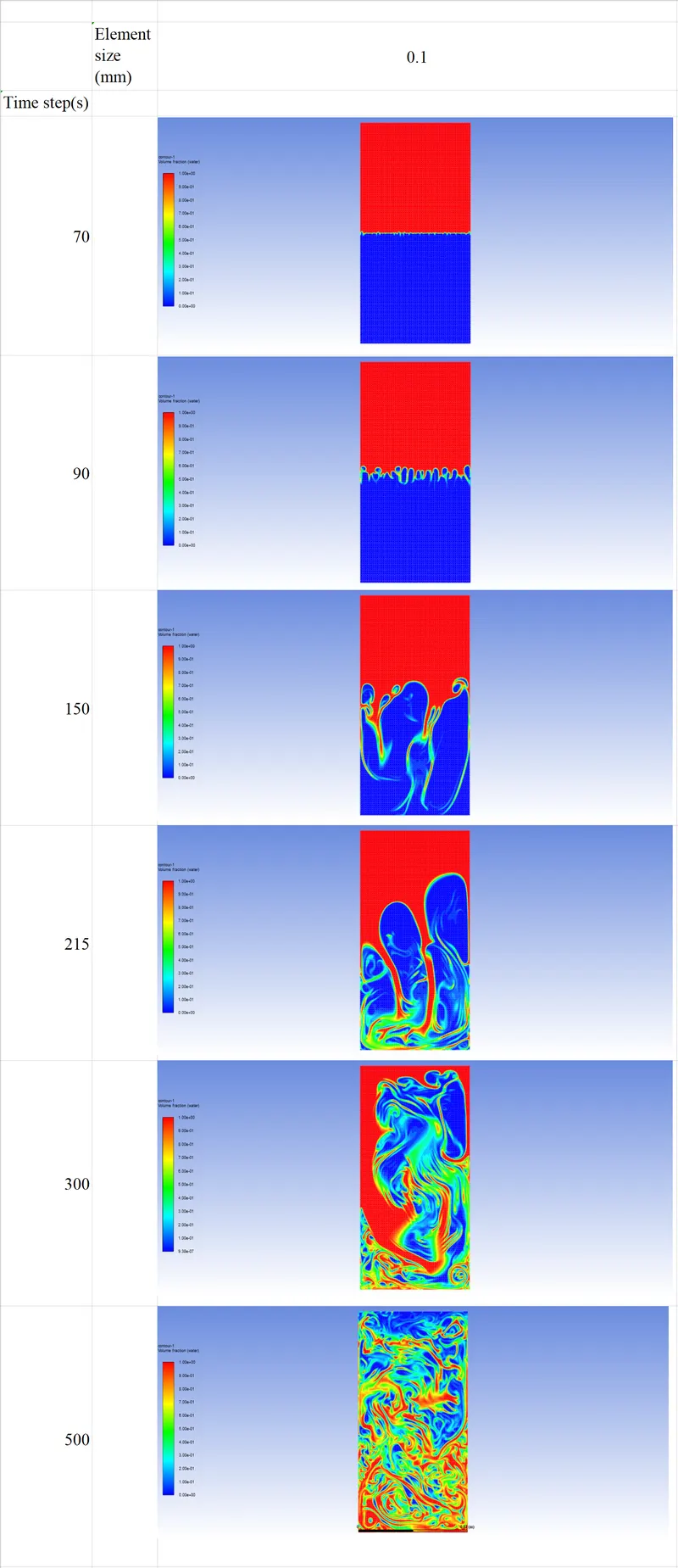
From the contours above, the behaviour of the Rayleigh-Taylor instability can be observed in detail.

At time-step 70, it can be seen that instabilities have begun to appear at the fluid interface. The heavier fluid(water), which is on top of the lighter fluid(air), begins to push into the air. The air phase is understandably unable to support the weight of the water phase. At time-step 90, water tendrils begin to penetrate into the air phase, and the growth of air bubbles begin as well. This is due to the potential difference between the two fluids. The density of water is significantly higher than that of air, and hence, the water phase possesses much greater potential energy. At time-step 150, the water tendrils grow longer, displacing a large amount of air in the process. The pressure of the air will play a vital role in this case, the water reduces the volume that the air can occupy, causing the formation of large bubbles or pockets of air. This can be seen clearly in the contour for time-step 215. At time-step 300, it can be seen that the water collides with the bottom wall, and hence, the velocity of the volume of water that has collided with the wall reduces significantly. Since the corners are occupied by slow moving water, the water that is moving toward it at a higher velocity experiences a tangential force at the boundary of the water that has slowed down, and hence, due to the viscosity of the air and this tangential force, rotational motion is introduced. This rotational motion causes the creation of turbulent eddies in the system, and vigorous mixing of air and water begins to take place. Eddies of different sizes can be seen throughout the domain. Turbulent eddies possess turbulent kinetic energy, and the eddies will interact with each other, reducing the amount of energy the have over time. At one point, the turbulent energy possessed by the eddies will dissipate, and the heavier fluid will settle at the bottom, while the lighter fluid will rest on top.

CASE I: Comparisons between mesh element sizes of 0.5, 0.2 and 0.1 mm

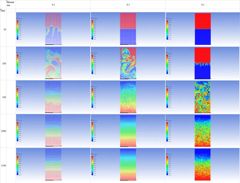
Observing the contours above, a few inferences can be drawn.

The results are highly dependent on the cell density. It can be seen that the results for the mesh with an element size of 0.5 mm converges and reaches steady state much faster than the other two cases. This is not desirable, as this does not accurately represent the actual behaviour of the fluid interface at a certain period of time. The time taken for the boundary to begin experiencing purturbations is significantly longer in the case with an element size of 0.1 mm. At time-step 100, the water tendrils just begin entering the air phase, whereas in the other two cases, turbulent mixing has already begun. Changing the element size has an effect on the time taken for the fluid to reach equilibrium. This is mainly due to fluid interactivity, and the nature of the model itself. The VOF model is somewhat binary in nature. A cell can either be water or air, but not contain both at the same time. If the element size is larger, it is clear that the cell will occupy more volume. The model will compute the momentum of a particular cell based on the momentum of the other cells(of their respective phases), and determine whether the cell contains water or air. Once this is done, it means that the area occupied by the cell contains only one particular phase. The area may contain multiple phases in reality, but since the element size is large, this is not accounted for. This also impacts phase interaction, as the number of cells containing their respective phases increases, and a larger number of eddies will be captured in the simulation. This, in turn, increases the amount of time the phases require to reach equilibrium.

Hence, it can be concluded that increasing the cell density of the domain will provide a more accurate representation of the phase interaction for the Rayleigh-Taylor waves.

CASE II: A user-defined fluid with a density of 400 `(kg)/(m^3)`, and a viscosity of 0.001 `(kg)/(m*s)`

The following volume fraction contours display the formation of the RT-instability at various time-steps, for a user-defined fluid and water.

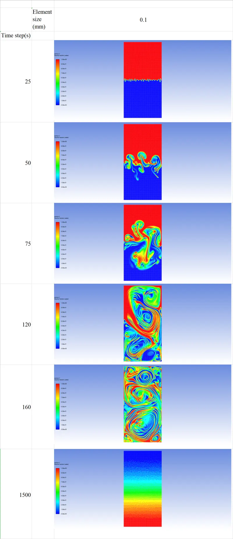
Observing the contours above, a few inferences regarding the density of the fluids are drawn.

The density of the light fluid phase plays a large role in the formation of the instability at the interface, in terms of the shape of the interface. In the previous case, it was observed that sharp tendrils of water penetrated the lighter air phase. If time-step 25 is observed for this case, the water penetration at the boundary appears more spherical in shape. It appears that the water penetrates the lighter phase with difficulty, compared to the previous case. In fact, the lighter fluid seems to form a mushroom like shape as the heavier fluid penetrates the interface, and this can be observed at time-step 50. The formation of eddies seems to occur due to a combination of inertial forces and viscous forces the fluids exert on each other. If time-step 75 is observed, these two forces can be seen to great effect. The water penetrates the interface, and proceeds to move downward, displacing the lighter liquid around it. However, in this case, the lighter fluid is denser than air. Since this fluid is heavier than air, this displaced fluid possesses more inertia, imparted to it due its displacement caused by the movement of water. The lighter fluid attempts to occupy the wake left by the penetrating water volume, and has enough force to cut off more water from entering that particular section. This movement is rotational in nature, and due to this, eddies are formed. The eddies that are formed in the fluid domain are easier to recognize in this case, and this can be attributed to the higher viscosity of the lighter fluid, displayed at time-step 160.

The time required for the fluid to reach steady state seems to have reduced as well. This can be attributed to the lower potential energy difference between the fluids. Since the density of the lighter fluid in this case is higher, the potential energy that is possesses is higher as well. Hence, ot can be stated that the density has an effect on the time required for the phases to reach steady state.

A steady-state simulation would not be optimal for this type of phenomena, as many of the subtle physical interactions that take place between the two phases would be lost. The Rayleigh-Taylor instability is highly time dependent, and understanding the differences between two different types of RT-instability with different fluid phase characteristics with respect to time would not be possible in a steady state simulation. Different types of fluid phases behave differently, and the interface instability occurs at different points of time due to this. A steady-state simulation would not take this into account.

Atwood number discussion:

The formulae for the Atwood number has been displayed below:

`A = (rho_1 - rho_2)/(rho_1 + rho_2)`

where,

`rho_1 = text(density of the heavier fluid)`

`rho_2 = text(density of the lighter fluid)`

Atwood number of air and water:

A = `(998.2 - 1.225)/(998.2 + 1.225) = 0.99754`

Atwood number of air and user-defined fluid:

A = `(998.2 - 400)/(998.2 + 400) = 0.4278`

The Atwood number describes the type of instability that can be expected from a domain containing fluids of two different densities. It can be seen that the Atwood number decreases with the increase in the density of the lighter fluid. Since the Atwood number is a quantity specific to Rayleigh-Taylor instabililities, it provides us with a metric that can be used to gauge the type of instability at the interface that can be expected when a heavy immiscible fluid is over a lighter fluid. It was seen that the types of RT-instabilities that were formed were very different in nature, despite having similar end results. Hence, it could be said that fluids with a high Atwood number will experience high turbulence, and the velocity of the fluid phases will be high as well. Fluids with a lower Atwood number will experience turbulent mixing as well, but the kinetic energy possessed by the eddies will be lower, as the density of the fluids are higher. The case with a low Atwood number will not have great heavy fluid acceleration during the beginning of the instability.

Hence, it can be concluded that turbulent mixing of two fluid phases will reduce as the Atwood number reduces.

Conclusion:

Observing the results, it can be concluded that the density of the mesh is influences the instability at the boundary greatly. Increasing the number of cells in a mesh will increase the amount of fluid interactions that take place(upto a certain limit), and as a consequence, the number of turbulent eddies that are formed in the system. High cell density is required to accurately capture the interface instabilities, and the actual number of spikes formed at the interface. The cell density influences the time required for the fluids to reach steady-state. The Atwood number describes the type of instability that can be expected from a domain containing fluids of two different densities, and will allow us to gauge the type of instability that can be expected from the two phases in question. It determines gives an idea of how the densities of two phases will affect the instability at the interface. As the Atwood number decreases, the instability at the interface will decrease, and vice versa. The density and viscosity of the fluids play a large role in the formation of eddies, as these two characteristics determine the potential energy difference between the two interacting fluids, and the energy that the turbulent eddies will possess.

Google drive link for animation files:

https://drive.google.com/drive/folders/1A5jJGUhAp-djqG_QmBPg2A3XKJMDpMVK?usp=sharing