The behaviour of different species after performing a combustion simulation, and the effect of the addition of water to fuel on the NOx and Soot formation

AIM: To observe the behaviour of different species after performing a combustion simulation, and the effect of the addition of water to fuel on the NOx and Soot formation.

Introduction and theory:

There are upwards of two hundred reactions that take place during the combustion of a hydrocarbon such as methane. The GRI-mech 3.0 mechanism, contains a total of three hundred and twenty-five reactions. Selecting the optimal fuel type for a specific situation requires a certain level of understanding of how the fuel would react under a varied range of conditions. Understanding a fuel's intrinsic behaviour with respect to reaction rate, temperature, and pressure are vital, and experimentation is necessary. Ascertaining the viability of fuel for combustion is largely dependent on the characteristics of the products after the combustion process is complete, and observing the behaviour of the fuel before, during and after the reactions take place. This can be done, by observing the behaviour of the flame produced due to combustion. The combustion of fuel, however, does result in the production of undesirable pollutants such as NOx and Soot. The production of the pollutants has a direct impact on the health of living creatures, as the production of Nitric Oxide and Nitrogen Dioxide can cause damage to the lungs, among other issues. Soot has a tendency of mixing with water bodies, and the atmosphere, and is also a contributor to global warming. The environment experiences the undesirable effects of these emissions, and for this reason, the production of these toxic chemicals must be regulated. The effect of mixing water with fuel on the production of these pollutants will be studied in detail in this project.

Simulation workflow:

Modelling and solving approach:

• Simulating combustion for an entire three-dimensional model would be highly expensive, and a large number of cells would inflate the simulation time. This can be avoided by taking advantage of the symmetric nature of the geometry. For this reason, a two-dimensional axisymmetric simulation will be performed. This will allow us to increase the number of cells and decrease the cell size in the geometry for maximum accuracy, without sacrificing too much computational speed.
• The species transport model will be used to simulate combustion. The species transport model does not contain a combustion model and does not contain reaction mechanisms. In reality, it is a transport equation. The species transport model solves the transport equations for different species. The basic gist of a transport equation is the calculation of the behaviour and quantity of a particular species within a control volume. This occurs due to advection and diffusion. The transport equation will use the concentration of the species as a variable and will compute the concentration of the species in the system. Fick's law will be used to compute species concentration. This model will allow us to track the formation of Soot and NOx in the system as well.
• In order to obtain the reaction rates of a reaction, the Eddy Dissipation model was used. This model uses turbulent mixing as the basis for computing the reaction rates. The reaction rates in this model depend on the dissipation rate of eddies. The turbulent energy possessed by an eddy will whittle down over time, eventually resulting in the formation of heat energy. This is most important factor about this model, as the rate at which the eddy dissipates will determine the rate at which combustion will take place, and is why the reaction rate and the eddy dissipation are intertwined. However, a turbulence model will be required in order for the Eddy Dissipation model to work, as turbulence is the foundation upon which this model is built. If the equation for the reaction rate for the Eddy Dissipation model is observed, it can be seen that it relies heavily on k(turbulent kinetic energy) and epsilon(dissipation rate).
• The k-epsilon turbulence model will be utilized in order to simulate the turbulent nature of the flow. The k-epsilon model is one of the simplest turbulence models available and is suitable for the current simulation.
• In order to obtain soot formation, a one-step soot-model(Khan and Greeves model) will be used. This model solves one transport equation, with the net rate of soot generation as the variable. This model is one of the simplest models available in fluent.

I) Geometry creation:

• The geometry was created using SpaceClaim. It should be noted that the geometry was created in the XY plane, as ANSYS Fluent requires that the direction of flow be along the X-axis for axisymmetric simulations.
• A plane was created, and the sketch tool was used to create the geometry.
• The geometry has been displayed below.

Geometry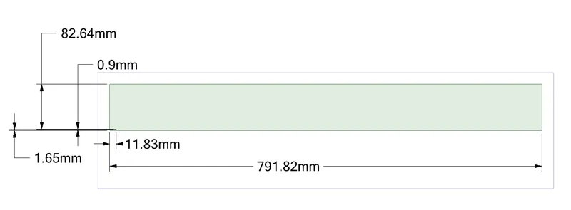

II) Mesh creation:

• After the geometry was imported into the Meshing module, the body was selected, and a mesh method was set as 'All triangles'.
• Two global settings were changed. The element size was changed to 1.8 mm, and the 'Capture Proximity' option was switched on.
• Under the 'Capture Proximity' settings, the number of cells along the gap was set to 5. This was done in order to provide an adequate number of cells to the fuel inlet, which is a very small opening.
• Appropriate named selections were provided for the fuel and air inlets, the outlet, and the axis of the geometry. The walls separating the fuel and air inlets were named as well.

Mesh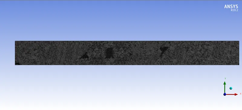
Fuel Inlet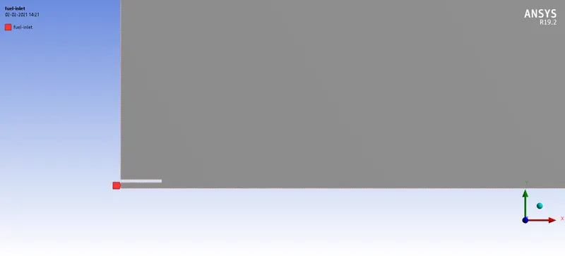
Air Inlet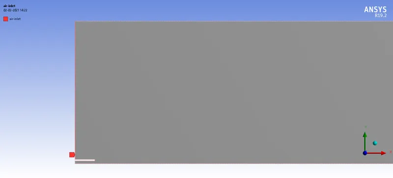
Axis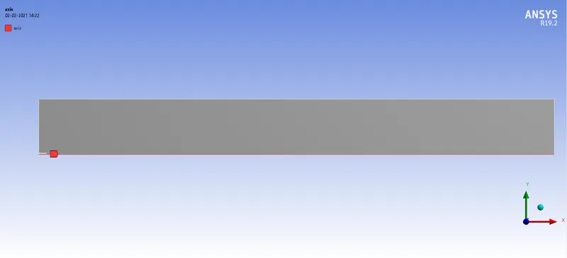
Walls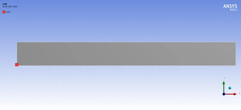

III) Fluent modelling:

(a) General settings:

• The simulations that are going to be carried out are steady-state in nature. This is set in the General section(Setup > General). Since the simulation is 2D-axisymmetric in nature, the Axisymmetric option under '2D-space' is switched on.

Solver used: pressure-based solver

A pressure-based solver is used for this case, as the compressibility effects are to be neglected. A density-based solver is highly accurate, but requires more computation time, and would not prove advantageous in this case. A pressure-based solver requires less computational time, and will provide accurate simulation results for this case. The pressure-based solver solves the governing equations in a sequence, unlike the density-based solver.

General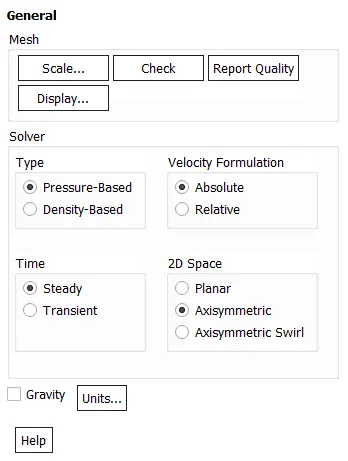

(b) Model settings:

(i) The energy equations are used by switching on 'Energy', in order to simulate the behaviour of heat in the combustor.

(ii) Model used : k-epsilon, with Standard wall-functions:

• The model that will be used in this simulation is the k-epsilon model. As mentioned above, the k-epsilon model will allow us to solve the turbulent kinetic energy(k) and dissipation rate(epsilon).
• Since the near-wall behaviour is not a priority, the standard wall functions have been used for this simulation.
• This has been done by entering Setup > Models > Viscous> k-epsilon > k-epsilon model.

Model settings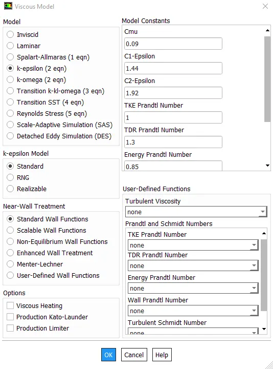

(iii) Species transport:

• The species model was set to 'Species Transport', by entering Models > Species.
• Under the 'Reactions' option, the 'Volumetric' option was switched on.
• Under the 'Options' section, the 'Inlet diffusion' and 'Diffusion energy source' options were switched on. This will allow us to compute the diffusion flux at the inlet, and the effect of transport due to the enthalpy of the species.
• The mixture material was set as Methane-air 2-step. This has been done in order to add `H_2O` to the fuel species.
• Under the 'Turbulence-chemistry' option, the Eddy Dissipation model was selected.

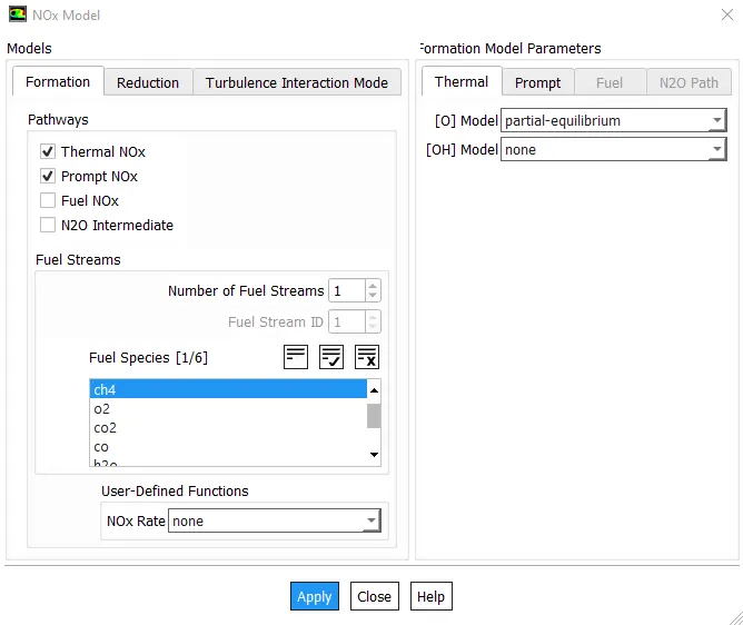
The transport equations for NOx and Soot were switched on by entering Models > Species > NOx, Soot.

NOx setup:

Formation:

• Under the Pathways section, Thermal NOx and Prompt NOx were switched on.
• Thermal NOx utilizes the extended Zeldovich mechanism, which computes the formation of thermal NOx. These reactions are temperature sensitive.
• The prompt NOx computes the formation of NOx in fuel-rich environments.
• Under Fuel Streams, the number of fuel streams was set to 1, and the fuel species was set to `CH_4`.
• The rest of the options were kept as their defaults.

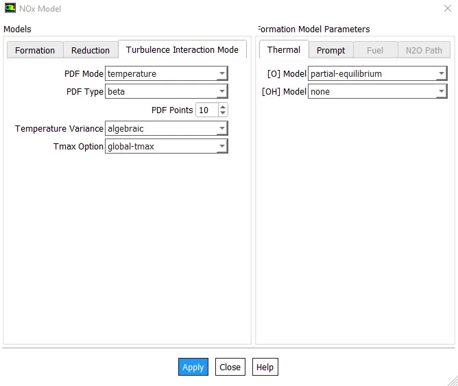
Turbulence Interaction Mode:

• The PDF mode and PDF type were set as 'temperature' and 'beta' respectively.
• The Temperature-variance was set to 'algebraic'

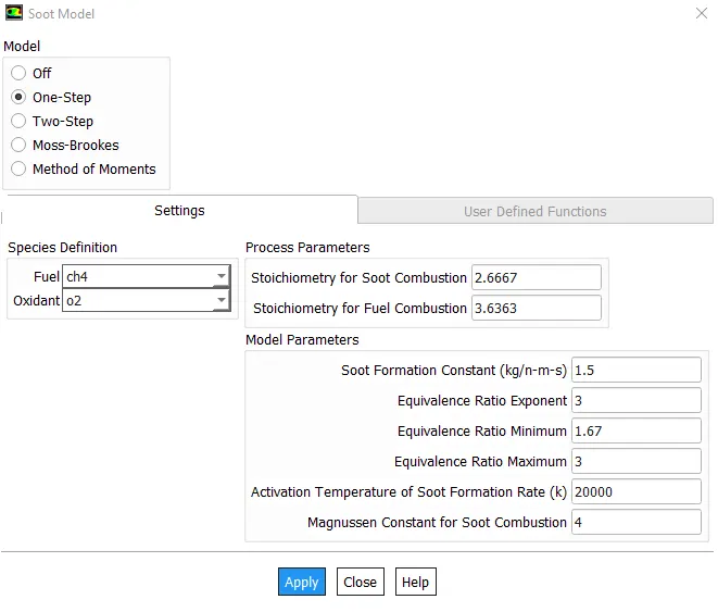
Soot setup:

• The One-step soot model was chosen for this simulation.
• The fuel was set to methane, and the oxidizer was set to oxygen. The other options were kept as their default values.

Species setup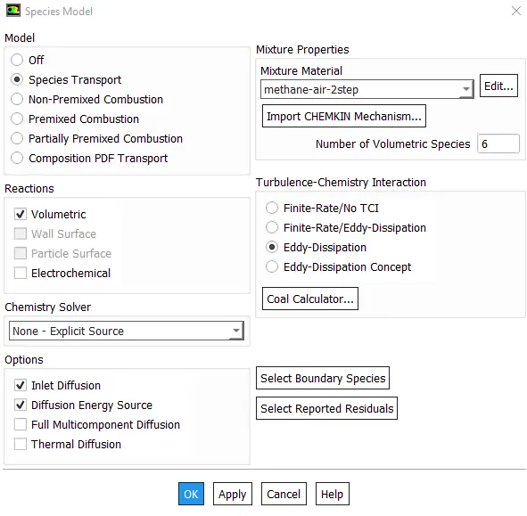

(c) Materials and Cell Zone Conditions:

• The fluid chosen for this simulation is air, and has been imported from the Fluent library by entering Setup > Materials > Fluid > Fluent Database.
• The mixture chosen for this simulation is methane-air two-step, the mixture is changed from the default to the newly imported fluid from the Fluent Database, methane-air 2-step.
• The working mixture in the fluid domain has been changed to methane-air 2-step by entering Cell Zone Conditions > 'fff_surface' > Material Name.

Materials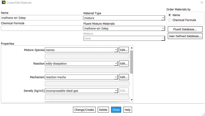
Cell Zone conditions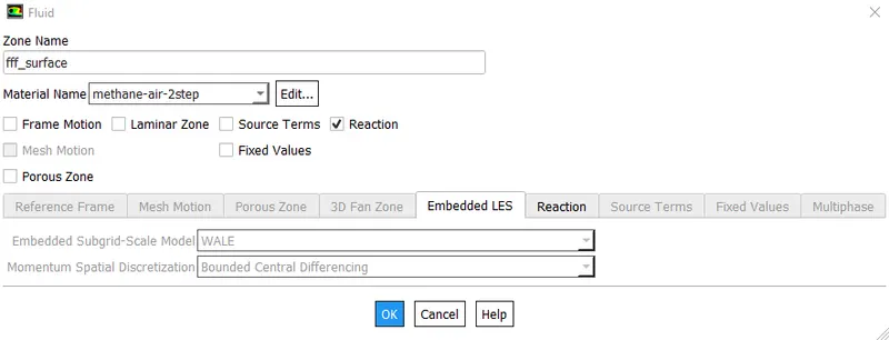

(d) Boundary conditions:

• The air inlet velocity is set to 0.5 m/s by entering Setup > Boundary Conditions > air-inlet. The species type is changed by entering the Species section, and setting a value of 0.21 as the mole fraction value for O2.
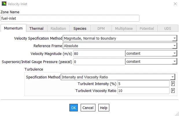
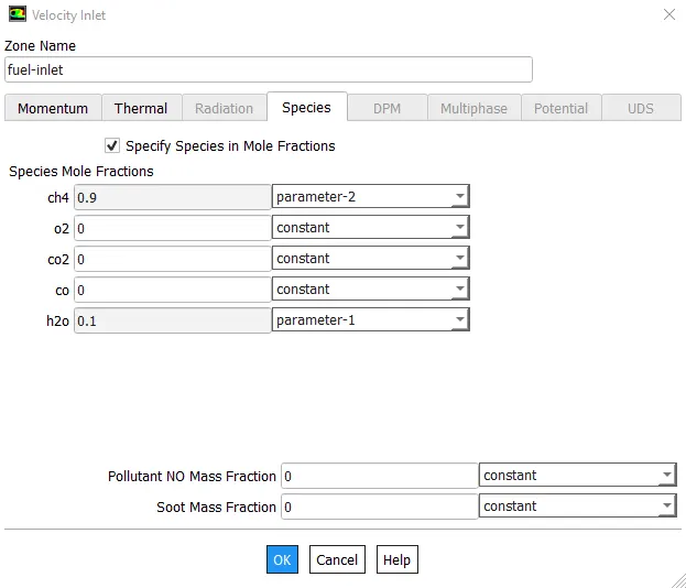
• The fuel inlet velocity is set to 80 m/s by entering Setup > Boundary Conditions > fuel-inlet. The species type is changed by entering the Species section. However, mole fractions of the species `CH_4` and `H_2O` are set as parameters that will be varied in the 'Parameter' section. Initially, the value of mole fractions of the species `CH_4` and `H_2O` are set to 1 and 0 respectively.
• The outlet is set to 'pressure-outlet'.
• The boundary conditions are set in Fluent, as shown in the table below.

• Location	Boundary condition
  Air Inlet	Velocity-inlet
  Fuel Inlet	Velocity-inlet
  Outlet	Pressure-outlet
  Wall	wall

• The number of iterations is set to 1800 by entering the value within the Run calculation section.

Boundary conditions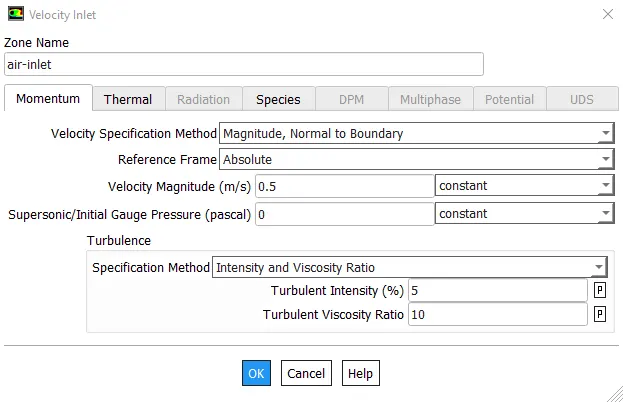

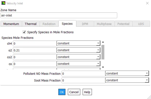(e) Method and Initialization settings:

• The turbulent kinetic energy and dissipation equations are solved using first-order upwind schemes, which will provide solutions with an accuracy of the first order (Solution > Methods).
• The species involved are solved using second-order upwind schemes.
• The solution is initialized by using Hybrid initialization by entering Solution > Initialization.

Methods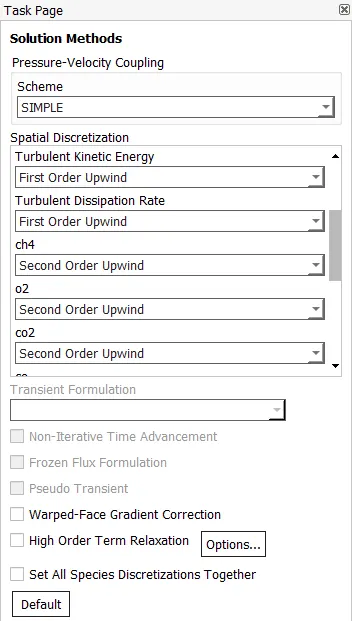

(f) Report generation:

• The NOx and Soot formation at the outlet were computed by creating a report for the area-weighted average of the mole fractions of NOx and Soot at the outlet.
• Within these report definitions, the 'Create Output Parameter' is selected, in order to monitor the output of these variables. This will allow us to plot the variation of the mole fractions of NOx and Soot with the change in the fuel mixed with water.

Report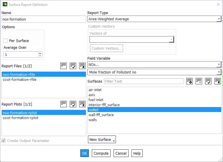

IV) Parameter Settings:

• The Parameter Set section was opened, where the required parameters were displayed, with their respective results. New Design points were created, providing different mole fraction values of water and fuel, in increments of 5 percent of the number of moles of the fuel.
• After these design points were created, each point was updated in order to obtain the required results of the parameters mentioned. These results were then exported into Microsoft Excel, where they were post-processed and the mole fractions of soot and `NO_x` were obtained and plotted on graphs, with respect to the water content in the fuel.

Parameter settings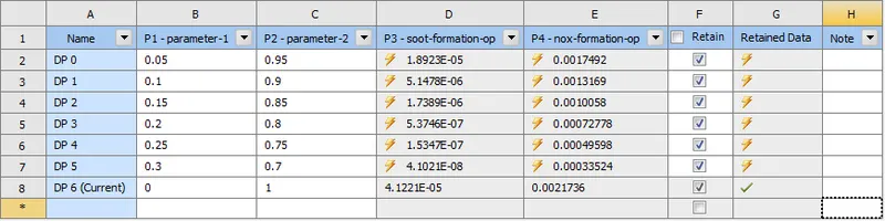

Results:

PART I : The behaviour of different species at different lengths along the X-axis

Vertical line probes were created at six locations along the X-axis, and have been displayed below.

Line probes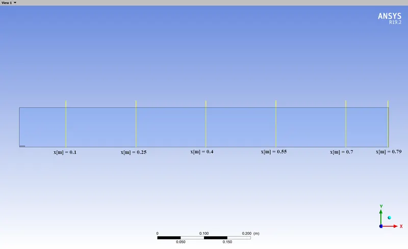

The following plots display the variation of the mass fractions of different species along the length of the line probe.

Species	Mass fraction
`CH_4`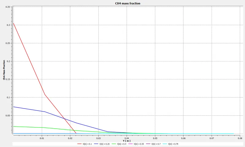
`O_2`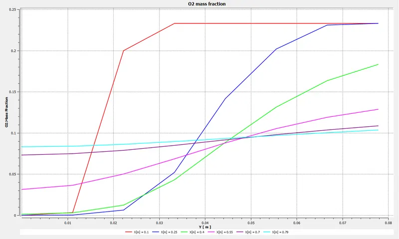
`H_2O`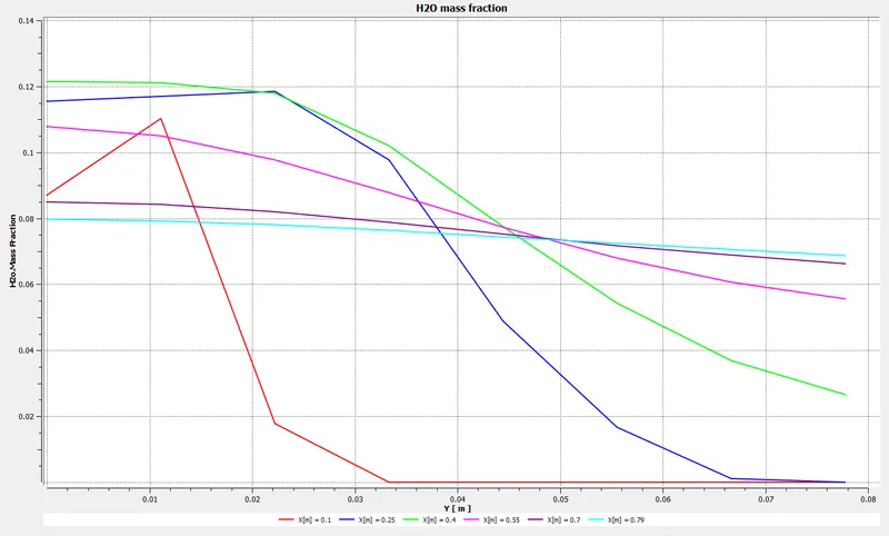
`CO_2`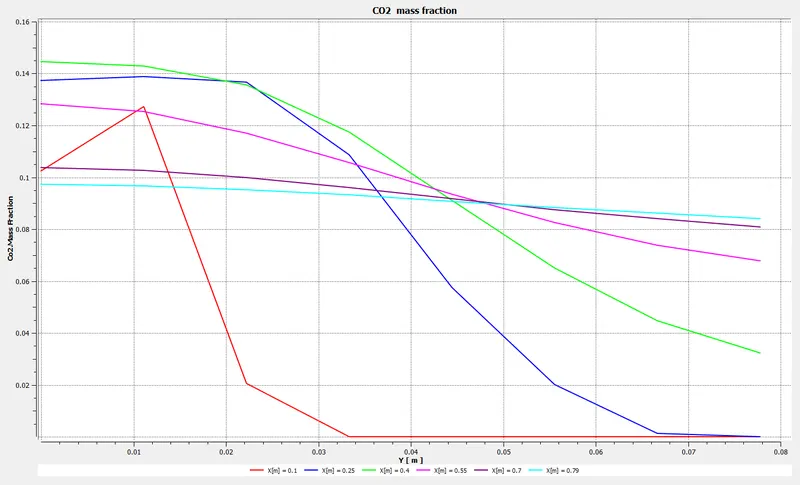
`NO_x`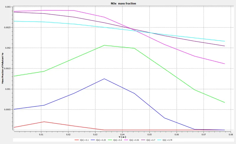
Soot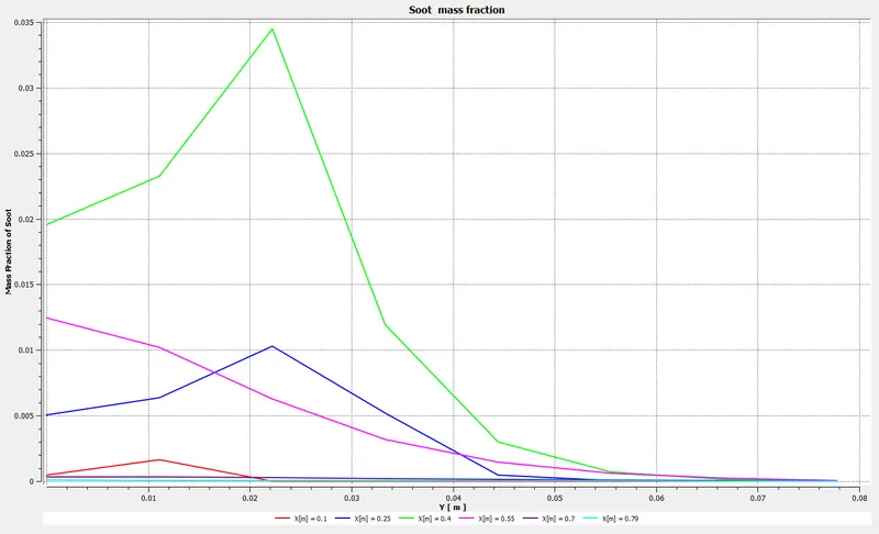

From the charts displayed above, a few inferences can be drawn.

If the chart for `CH_4` is observed, it can be seen that the mass fraction `CH_4` reduces as the domain length increases, until it is completely consumed at the outlet. This was the expected outcome, as the fuel will react with the air at the inlet, to form the main products carbon dioxide and water, and some minor products. If the plot is observed in detail, it can be seen that the concentration of `CH_4` exists only under a certain height in the domain. This means that it is consumed some short distance from the axis of the domain, and does not spread to the outer boundaries.

Observing the chart for the mass fraction of `O_2`, it can be seen that the oxygen entering through the air inlet is consumed as the domain length increases. However, the concentration of `O_2` increases in the areas near the axis, after 0.55 m. This suggests that combustion occurs at some point before this, and the `O_2` entering the inlet is not completely consumed. This also means that the concentration of fuel is so low or non-existent, combustion does not take place beyond this point. This behaviour will be explained in detail below.

The Eddy Dissipation model is based on turbulent mixing. Turbulent mixing occurs due to the mixing of the fuel and the air. This creates turbulent eddies in the system, and the rate at which the eddies dissipate or lose their kinetic turbulent energy, determines the rate of reaction, i.e, combustion. If the turbulent mixing is not taking place, this means that combustion is not taking place. At some point, the fuel is completely consumed, and there is no fuel for the air to react with. So, the mass fraction of the air near the area around the axis after 0.55 m, begins increasing.

The increasing quantity of oxygen does have an effect on the products created and will be discussed later in this section.

If the chart for `H_2O` is observed, it re-enforces the point that has been previously made. The mass fraction of `H_2O` is the highest at 0.4 m, and then gradually begins reducing. This suggests that in this region, maximum combustion takes place, and as the mass fraction of the fuel reduces after this region, the amount of `H_2O` produced reduces as well. The same trend can be observed in the chart containing the concentration of `CO_2`.

Production of `NO_x` and Soot:

Observing the chart for `NO_x`, it can be seen that the mass fraction of `NO_x` begins increasing after 0.55 m. It has been established that the combustion is at its peak before this point, around 0.4 m. But the concentration of `NO_x` continues increasing greatly, after peak combustion. This occurs due to the points mentioned above. The out of the two pathways of `NO_x` formation, it is known that the thermal `NO_x` pathway produces much more `NO_x`. This occurs due to the lack of combustion of air with the fuel. The temperature of the air easily exceeds temperatures of 2000 K in the regions surrounding the peak combustion zone, and the unreacted `O_2` begins reacting with `N_2`, resulting in the production of `NO_x`. It should be noted that thermal `NO_x` production occurs only when the temperature is high and is less prevalent in low-temperature combustion. The Zeldovich mechanism generates a high amount of `NO` when the temperature of air exceeds 1570 K, and this is the main reason the production of `NO_x` is this high. The mixture of air and fuel become significantly leaner at the end of the combustor, and hence, the production of `NO_x` is high.

Soot formation occurs due to incomplete combustion. Soot is formed due to lack of oxygen. Observing the chart for the mass fraction of soot, it can be seen that soot formation is maximum where the combustion seems to be the highest, at around 0.4 m. This is logical, as the amount of fuel available after this point is extremely low, and soot formation will occur when the fuel is still available. The mass fraction of soot reduces after 0.4 m, for the reason stated above. Nevertheless, the formation of soot is an undesirable phenomenon.

The following images display the temperature, mass fractions of `NO_x` and soot contours of the domain for this case. These contours re-enforce the points made above.

Contours	Domain
Temperature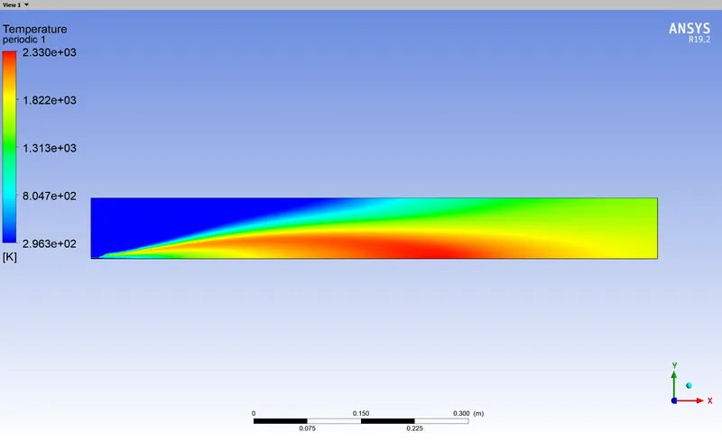
Mass fraction of `NO_x`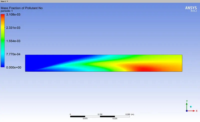
Mass fraction of Soot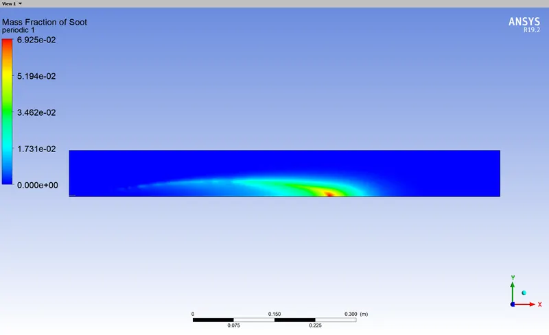

The effect of mixing water with the fuel on the `NO_x` and soot formation will be observed below.

PART II: Observing the effect of varying quantities of water in the fuel on `NO_x` and soot generation

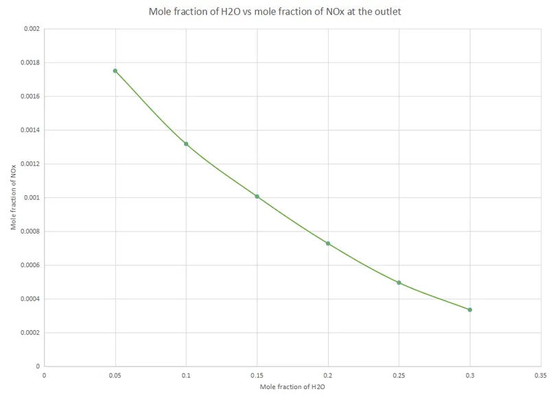
After conducting a parametric study of the effect of varying quantities of water in the fuel on `NO_x` and soot generation, the following plots were obtained.

Species	Plots
Mole fraction of `H_2O` vs mole fraction of `NO_x` at the outlet
Mole fraction of `H_2O` vs mole fraction of soot at the outlet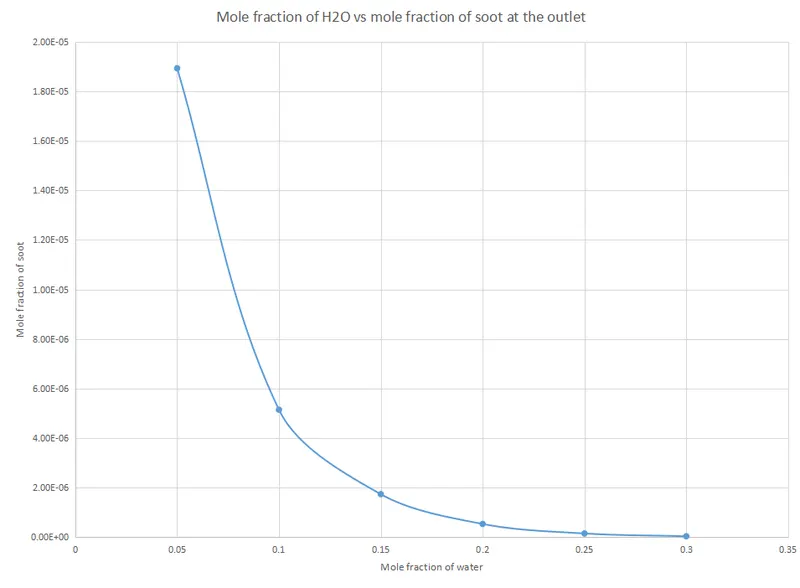

Observing the plots shown above, it can be seen that the mole fraction of soot and `NO_x` at the outlet reduce drastically with the addition of water in the fuel.

The reason this inhibits the production of `NO_x` so greatly, is due to the fact that the water in the fuel, directly and indirectly, interacts with the excess air that is leftover after peak combustion takes place. As previously mentioned, the peak combustion region renders the region beyond it devoid of fuel content, and this leads to the formation of `NO_x`. This issue is avoided to a great degree with the addition of water in the fuel. A high amount of `OH` is created as a result of the chemical interactions between `H_2O` and `O_2`. However, the extended Zeldovich mechanism contains a reaction in which `OH` may lead to the production of `NO_x`(`N + OH leftrightarrow H + NO`), and this may lead to the argument that this process is counter-intuitive. But, this is not the case, as the `OH` present interrupts one of the main reactions that create `NO`(`O + N_2 leftrightarrow N + NO`). The `OH` that is created by the chemical interactions between `O_2` and `H_2O` reacts with the `N_2` mentioned in the previous reaction. The `N_2` prefers reacting with the `OH`, instead of the monoatomic oxygen, and creates nitrous oxide instead(`OH +N_2O+O leftrightarrow N_2O + OH`).

This is the main reason why the production of `NO_x` reduces.

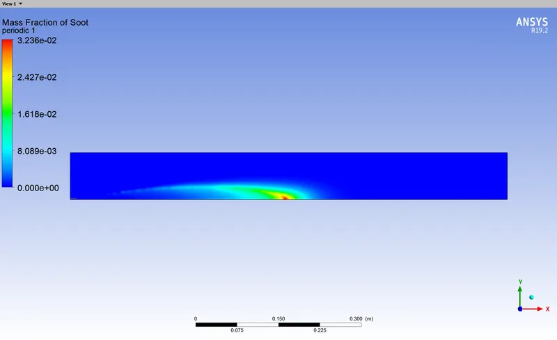
The following contours of the mass fractions of `NO_x` and soot display the behaviour mentioned above.

Mole fraction of water	`NO_x`	Soot
0.05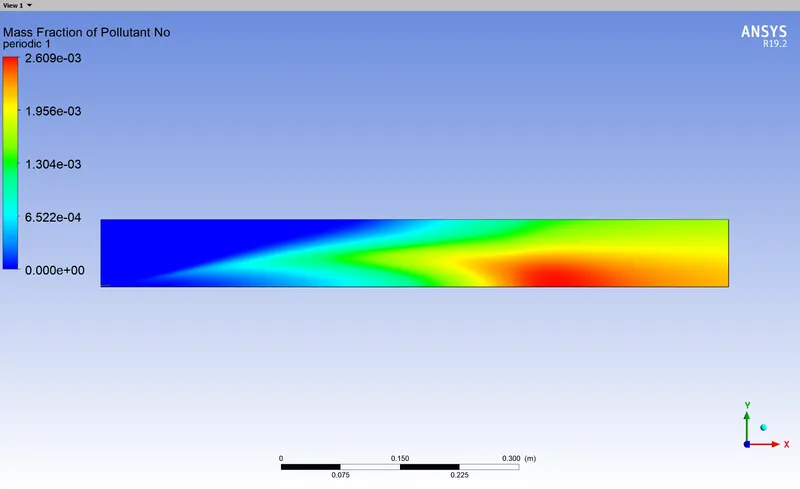
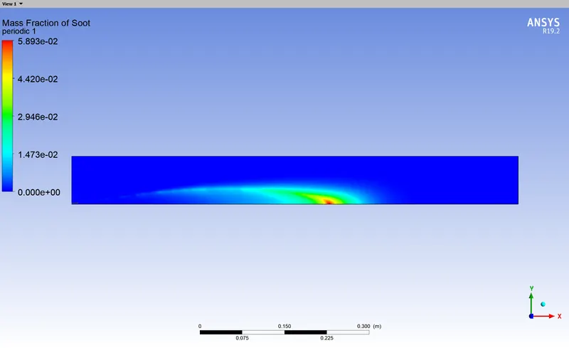0.2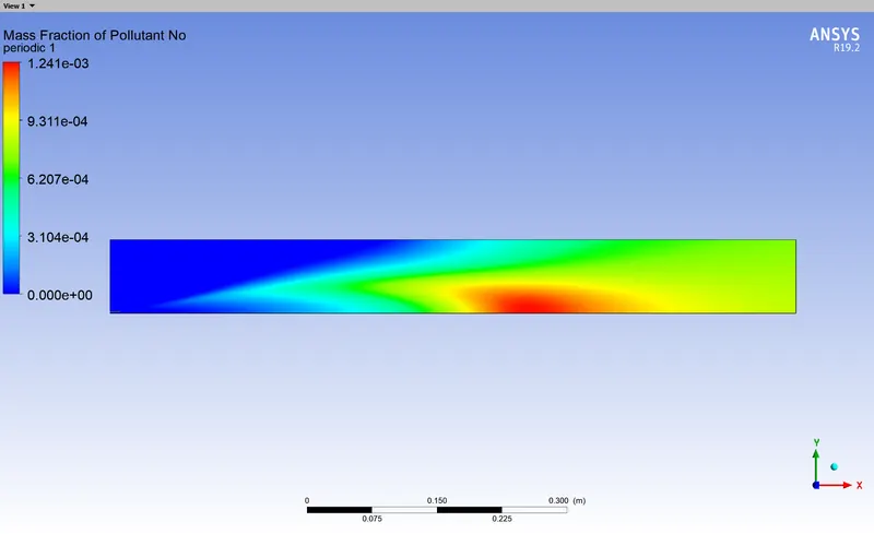
0.3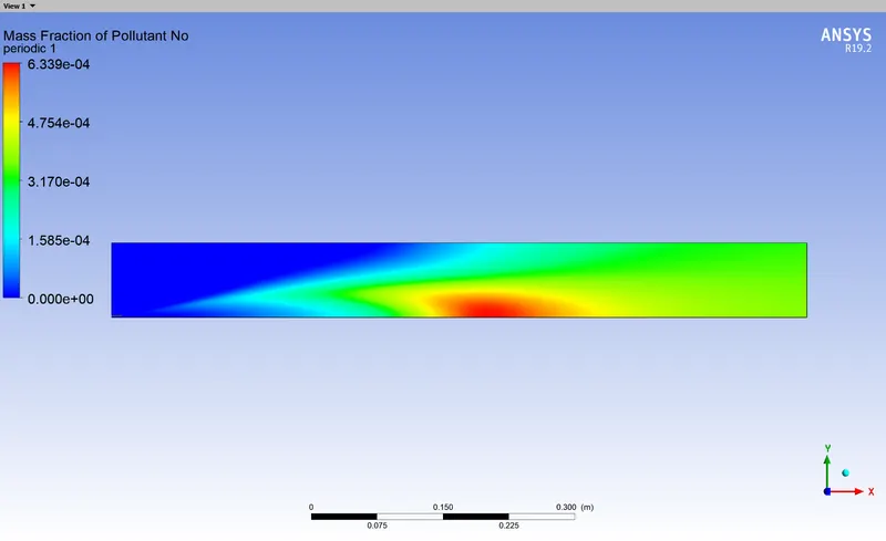

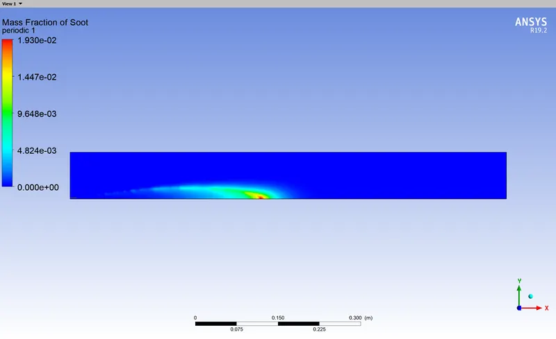From the contours above, it can be observed that the mass fraction `NO_x` reduces significantly as the amount of water in the fuel increases. The concentration of `NO_x`along the domain length reduces and a majority of the excess air is consumed. The Soot formation is reduced as well, as the water in the fuel promotes more mixing of the fuel with air, by virtue of an increased auto-ignition delay time. The autoignition delay time is the time the mixture takes to ignite, without external heat inducement. The area within which soot formation takes place reduces significantly, and this can be observed in the contours as well.

Hence, it can be concluded that increasing the water content in the fuel reduces the amount of `NO_x` and soot produced during combustion significantly.

However, this does come at a cost. The following temperature contours display the drawbacks that will be mentioned in the section below.

Mole fraction of water	Temperature contours
0.05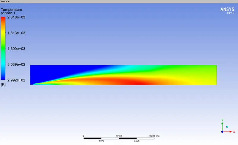
0.2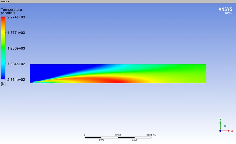
0.3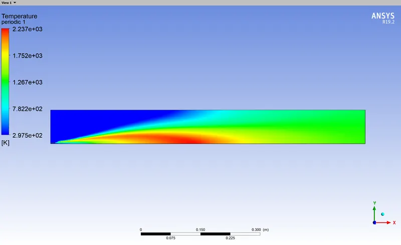

From the contours displayed above, it can be observed that the max temperature that can be achieved after combustion reduces significantly. The max temperature that is achieved without the addition of water is 2330 K, while the max temperature achieved by the fuel with 30 percent water is 2237 K, a 100 K temperature drop. Hence, the amount of water that should be added to the fuel needs to be varied according to the objective at hand. Increasing the amount of water in the fuel beyond a certain value will most definitely affect the efficiency of the combustor.

Conclusions:

From the results shown above, it can be concluded that the formation of `NO_x` is directly affected by the amount of oxygen present in the system after peak combustion. The high-temperature oxygen that remains unreacted after combustion promotes the Zeldovich mechanism, which creates `NO_x` due to the thermal `NO_x` formation pathway. The soot formation occurs in the area around the peak combustion region, due to lack of oxygen. This issue can be mitigated by adding water to the fuel. Increasing the mole fraction of the water in the fuel will decrease the amount of `NO_x` and soot that is produced after combustion, by increasing the auto-ignition delay time. This allows for increased fuel mixing. The water in the fuel and the unreacted high-temperature oxygen react, creating `OH`, and hence reduce the amount of oxygen that can react with the nitrogen in the system. However, the reduction in the production of `NO_x` and soot comes at the cost of capping the max temperature to a reduced value. A 100 Kelvin drop in the maximum temperature was observed, and hence, it can be said that there is essentially a trade-off to be made between pollutant reduction and combustor efficiency.