Simulating the phenomenon of auto-ignition of an air-fuel mixture using the Cantera library.
AIM:
(1)To observe the variation of the Auto-ignition time of Methane with varying initial temperature and pressure conditions.
(2)To observe the rate of change of molar concentration of the species present in the combustion reaction, with varying temperature and pressure conditions.
Introduction:
Observing the behaviour and characteristics of a fuel is important, as this provides an insight into it's utility. This is important, as it allows us to gauge which fuel is optimal for a specific purpose or situation. The auto-ignition delay time is the time taken by the fuel to combust, without an external provision for heat. This is the lowest possible temperature at which combustion can take place. Auto-igniton depends on different factors such as initial temperature of the fuel and pressure. The variation of auto-ignition delay times and temperatures with change in temperature and pressure will be observed in the sections below.
Theory:
The effects of auto-ignition are case dependent. In some cases, auto-ignition is a favourable phenomenon, while in some cases, it is an unfavourable phenomenon. The most notable case of unfavourable auto-ignition, is present in spark-ignition engines. In many cases, knocking in a spark-ignition engine is attributed to auto-ignition in the fuel. This occurs when the unburnt high temperature combustion products are still present in the combustion chamber. This causes combustion, without the activation of the spark, and the piston at this point, has not completed it's compression stroke. The pressure in the combustion chamber increases rapidly, and a force is exerted on the piston, opposing it's movement to the top of the combustion chamber. This can have detrimental effects on the piston itself, and it will incur significant damage due to the production of pressure pulses in the combustion chamber. Hence, obtaining the auto-ignition temperature of the fuel is important, and preventive measures can be taken to mitigate this issue.
Auto-ignition in a diesel engine however, is a favourable phenomenon. The diesel engine works on the concept of auto-ignition, as there is no spark plug present. In the combustion chamber, after a sufficient value of temperature is achieved, the elevated temperature of the mixture becomes significant, and causes the mixture to combust. Hence, knowing the autoignition temperature of a fuel becomes vital in this case.
Formulae used:
Ignition delay time:
`t_text(ignition delay) = t_text(initial temperature + 400K)`
`text(where,)`
`t_text(ignition delay) = text(time required for auto-ignition)`
Coding Approach:
The following steps were performed to achieve the required objectives:
PART I:
Step I: Importing libraries, setting initial conditions
- The sys, Cantera, NumPy and matplotlib libraries were imported into the program.
- The initial ranges of temperatures and pressures required, were set using the 'arange' function of the NumPy library.
- The number of timesteps and the time increment were set. There are two sets of these values and the use of these two sets of values will be elaborated upon in the next section.
- The pressure in Cantera is computed in Pascals, so the required conversion has been performed in the code.
Lines of code:
import sys
import numpy as np
import cantera as ct
import matplotlib.pyplot as plt

#PART I:

#Temperature:
T   = np.arange(950,1650,100)

#Pressure in atm:
atm = np.arange(1,7,1)

#Pressure in pascal
P   = atm*101325

#Number of time steps and time increment value:
n_timesteps = 1e5
time_inc    = 1e-4

#Number of time steps and time increment value: [for higher accuracy]
n_timesteps_prec = 1e8
time_inc_prec    = 1e-7
Step II: Defining functions
- Two functions have been created. The first function will simulate the auto-ignition over a period of 10 seconds. The second function is similar to the first function, but will provide more precise values for auto-ignition delay time.
- The function takes initial temperature, pressure, time increment, and number of time steps as required input arguments.
- Within the function, a gas object is defined by using the Solution class in cantera. This class is used to compute the reactions of the species present in a mixture or a solution in general. The 'gri30.xml' file has been imported using this class. GRI-Mech 3.0 is a mechanism used to deal with the combustion of fuels.
- The initial temperature, pressure and number of moles of the gas object are defined using 'TPX'.
- An ideal gas reactor model has been chosen for this simulation, and the 'IdealGasReactor' class has been utilzed for this purpose. This behaves like a constant volume combustion chamber, with no heat loss present at the boundaries, and no work is done in the chamber itself.
- A reactor network is defined by using the 'ReactorNet' class. The instance of the reactor model defined above is taken as an input argument, and this allows us to simulate the reaction over a period of time.
- The thermodynamic state of the system is defined by using the 'SolutionArray' class, which returns the thermodynamic state of the gas object or mixture at a specific time as multiple arrays.
- A 'for' loop is defined within the function, and is used to define the number of time steps over which the simulation is to be performed. Inside the loop, the time increment is defined. The time increment is the time at which a solution for the thermodynamic state is required.
- The 'advance' function is used to integrate the function with respect to the time increment specified.
- The thermodynamic states of the chemical reactions at a particular time are added to their respective arrays(the Solution Array defined above), by using the 'append' function.
- Finally, the function is set to return the thermodynamic states of the species at the specified time.
- The second function is mostly identical to the first function, but uses a smaller time increment and a greater number of time steps. This is used to obtain a more precise auto-ignition delay time, for the specified conditions. An 'if' loop is created inside the 'for' loop inside this function. If the auto-ignition temperature is reached or exceeded, the value of the auto-ignition delay time will be printed and the loop will break after this criterion is satisfied. The criterion has been specified in the Theory section above. This function returns the thermodynamic state of the mixture at a specific time, similar to the first function.
Lines of code:
#functions to find T,P,and mole fractions:
def auto_ignition(T,P,n_timesteps,time_inc):

	gas     = ct.Solution('gri30.xml')
	gas.TPX = T,P,{'CH4':1,'O2':2,'N2':7.52}
	r       = ct.IdealGasReactor(gas)
	sim     = ct.ReactorNet([r])
	time    = 0.0
	states  = ct.SolutionArray(gas,extra = ['t'])

	for n in np.arange(n_timesteps):
		time += time_inc
		sim.advance(time)

		states.append(r.thermo.state,t = time)

	return states

def auto_ignition_exact(T,P,n_timesteps,time_inc):

	gas     = ct.Solution('gri30.xml')
	gas.TPX = T,P,{'CH4':1,'O2':2,'N2':7.52}
	r       = ct.IdealGasReactor(gas)
	sim     = ct.ReactorNet([r])
	time    = 0.0
	states  = ct.SolutionArray(gas,extra = ['t'])

	for n in np.arange(n_timesteps_prec):
		time += time_inc_prec
		sim.advance(time)

		if(r.T>=T+400):
			A = print('Auto-ignition delay(T = '+str(T)+' K'+',P = '+str(P)+' Pa) = ' + str(sim.time)+' s')
			break

		states.append(r.thermo.state,t = time)

	return states
Step III: Obtaining the auto-ignition delay time
Constant pressure, varied temperature:
- A 'for' loop is created, using the total number of temperature values for which the thermodynamic states of the mixture are required, as the range of the loop. This has been done by using the 'len' function, that will return the total number of items inside a list, and the 'arange' function of the NumPy library.
- The two functions mentioned in the previous step are inserted into the loop. The first function utilizes a reduced number of time steps and a larger time increment. The pressure has been kept constant for this loop, and the temperature is varied from 950 K to 1450 K. Hence, after every run of the loop, a new value of temperature will be used from the range specified above.
- The second function that has been inserted uses a higher number of time steps and a smaller time increment. This has been done to achieve more precise values of auto-ignition delay times. This will print the exact auto-ignition delay time in the console.
- The plotting commands have been inserted in the loop as well, and will be discussed at the end of this section.
Constant temperature, varied pressure:
- The procedure followed to obtain the thermodynamic state of the mixture is the same as above, with two main differences. The 'for' loop utilizes the range of pressure values between 1 to 5 atm, while keeping the temperature constant at 1250 K.
- Again, the two functions mentioned above are utilized, and use the varied pressure values mentioned above.
Plotting and plotting functions used:
The plot uses string concatenation to create the legend. After each run of the 'for' loop, the 'str' function converts the value of temperature and pressure that it is currently utilizing for computation, into string format. This allows us to automatically use these variable values, without manual input.
- title: Used to provide a title to the plot.
- plot: Used to create a simple line plot. The 'label' argument is used to create a label for the plot to be used in the legend.
- xticks,yticks: Provides a range of values to be used on the X and Y axes respectively. The 'arange' function has been used within this function to introduce float values within the range.
- xlabel,ylabel: Used to name the X and Y axes respectively.
- legend: Creates the legend for the plot.
- show: Displays the plot.
Lines of code:
print('PART I:')
print('Constant Pressure,varying temperature: ' )

for i in np.arange(1,len(T)):

	C_pre     = auto_ignition(T[i-1],P[4],n_timesteps,time_inc)
	C_pre_exa = auto_ignition_exact(T[i-1],P[4],n_timesteps_prec,time_inc_prec)

	plt.figure(1)
	plt.xticks(np.arange(0,11,0.5))
	plt.yticks(np.arange(950,5000,50))
	plt.xlabel('Simulation time(s)')
	plt.ylabel('Temperature(K)')
	plt.title('Simulation time(s) vs Temperature(K) : [Constant initial pressure]')
	plt.plot(C_pre.t,C_pre.T,label= 'Initial temperature = ' + str(T[i-1]) + 'K')
	plt.legend()

	plt.figure(2)
	plt.xticks(np.arange(0,1,0.02))
	plt.yticks(np.arange(950,5000,50))
	plt.xlabel('Auto-ignition delay time(s)')
	plt.ylabel('Temperature(K)')
	plt.title('Auto-ignition delay time(s) vs Temperature(K) : [Constant initial pressure]')
	plt.plot(C_pre_exa.t,C_pre_exa.T,label= 'Initial temperature = ' + str(T[i-1]) + 'K')
	plt.legend()

print('n')
print('Constant temperature,varying Pressure: ')

for j in np.arange(1,len(P)):

	C_temp     = auto_ignition(T[3],P[j-1],n_timesteps,time_inc)
	C_temp_exa = auto_ignition_exact(T[3],P[j-1],n_timesteps,time_inc)

	plt.figure(3)
	plt.xticks(np.arange(0,11,0.5))
	plt.yticks(np.arange(950,5000,50))
	plt.xlabel('Simulation time(s)')
	plt.ylabel('Temperature(K)')
	plt.title('Simulation time(s) vs Temperature(K) : [Constant initial temperature]')
	plt.plot(C_temp.t,C_temp.T,label= 'Initial pressure = ' + str(P[j-1]) + ' Pa')
	plt.legend()

	plt.figure(4)
	plt.xticks(np.arange(0,0.05,0.001))
	plt.yticks(np.arange(950,5000,50))
	plt.xlabel('Auto-ignition delay time(s)')
	plt.ylabel('Temperature(K)')
	plt.title('Auto-ignition delay time(s) vs Temperature(K) : [Constant initial temperature]')
	plt.plot(C_temp_exa.t,C_temp_exa.T,label= 'Initial pressure = ' + str(P[j-1]) + ' Pa')
	plt.legend()

print('n','n'+'PART II:')
PART II:
Step IV: Obtaining the molar concentrations of O2,H2O,OH:
- The molar concentrations of the required species are obtained in this part.
- The molar concentration of the species at temperatures of 500 K and 1000 K are required, and have been defined using the 'arange' function. A constant initial pressure of 5 bar for both cases has been defined as well.
- A 'for' loop is created, using the total number of temperatures specified in the range as the total number of loops that will be run, using the 'len' function. Within the loop, the first function has been used to obtain the thermodynamic states of the mixture, over a period of 10 seconds(specified within the function).
- In order to obtain the molar concentration of the species, the 'concentrations' function will be used, along with the 'species_index' function. The 'concentrations' function will return the molar concentration of the species in `(kmol)/m^3`. The 'species_index' function will sift through the array in order to obtain the molar concentration of the species required specifically.
- The same plotting commands were utilized to obtain the plots in this section.
Lines of code:
#PART II:
T_mol = np.arange(500,2000,500)

P_mol = 500000
for k in np.arange(1,len(T_mol)):
	St_mol  = auto_ignition(T_mol[k-1] ,P_mol,n_timesteps,time_inc)


	O2  = St_mol.concentrations[:,St_mol.species_index('O2') ]
	H2O = St_mol.concentrations[:,St_mol.species_index('H2O')]
	OH  = St_mol.concentrations[:,St_mol.species_index('OH') ]

	print('Molar concentration of O2 (kmol/m^3)(T = '+str(T_mol[k-1])+' K,P = ' +str(P_mol)+' Pa):'+'n'+str(O2 )+'n')
	print('Molar concentration of H2O(kmol/m^3)(T = '+str(T_mol[k-1])+' K,P = ' +str(P_mol)+' Pa):'+'n'+str(H2O)+'n')
	print('Molar concentration of OH (kmol/m^3)(T = '+str(T_mol[k-1])+' K,P = ' +str(P_mol)+' Pa):'+'n'+str(OH )+'n')
	plt.figure()
	plt.title('Auto-ignition delay time(s) vs molar concentrations : [Constant initial pressure]')
	plt.ylabel('Molar concentration(kmol/m^3)')
	plt.xlabel('Simulation time(s)')
	plt.xticks(np.arange(0,11,0.3))
	plt.yticks(np.arange(0,1,0.001))
	plt.plot(St_mol.t,O2, label=' molar concentration of O2 (kmol/m^3)'+' (T= '+str(T_mol[k-1])+')')
	plt.plot(St_mol.t,H2O,label=' molar concentration of H2O(kmol/m^3)'+' (T= '+str(T_mol[k-1])+')')
	plt.plot(St_mol.t,OH, label=' molar concentration of OH (kmol/m^3)'+' (T= '+str(T_mol[k-1])+')')
	plt.legend()

plt.show()
Code:
import sys
import numpy as np
import cantera as ct
import matplotlib.pyplot as plt

#PART I:

#Temperature:
T   = np.arange(950,1650,100)

#Pressure in atm:
atm = np.arange(1,7,1)

#Pressure in bar
P   = atm*101325

#Number of time steps and time increment value:
n_timesteps = 1e5
time_inc    = 1e-4

#Number of time steps and time increment value: [for higher accuracy]
n_timesteps_prec = 1e8
time_inc_prec    = 1e-7

#functions to find T,P,and mole fractions:
def auto_ignition(T,P,n_timesteps,time_inc):

	gas     = ct.Solution('gri30.xml')
	gas.TPX = T,P,{'CH4':1,'O2':2,'N2':7.52}
	r       = ct.IdealGasReactor(gas)
	sim     = ct.ReactorNet([r])
	time    = 0.0
	states  = ct.SolutionArray(gas,extra = ['t'])

	for n in np.arange(n_timesteps):
		time += time_inc
		sim.advance(time)

		states.append(r.thermo.state,t = time)

	return states

def auto_ignition_exact(T,P,n_timesteps,time_inc):

	gas     = ct.Solution('gri30.xml')
	gas.TPX = T,P,{'CH4':1,'O2':2,'N2':7.52}
	r       = ct.IdealGasReactor(gas)
	sim     = ct.ReactorNet([r])
	time    = 0.0
	states  = ct.SolutionArray(gas,extra = ['t'])

	for n in np.arange(n_timesteps_prec):
		time += time_inc_prec
		sim.advance(time)

		if(r.T>=T+400):
			A = print('Auto-ignition delay(T = '+str(T)+' K'+',P = '+str(P)+' Pa) = ' + str(sim.time)+' s')
			break

		states.append(r.thermo.state,t = time)

	return states

print('PART I:')
print('Constant Pressure,varying temperature: ' )

for i in np.arange(1,len(T)):

	C_pre     = auto_ignition(T[i-1],P[4],n_timesteps,time_inc)
	C_pre_exa = auto_ignition_exact(T[i-1],P[4],n_timesteps_prec,time_inc_prec)

	plt.figure(1)
	plt.xticks(np.arange(0,11,0.5))
	plt.yticks(np.arange(950,5000,50))
	plt.xlabel('Simulation time(s)')
	plt.ylabel('Temperature(K)')
	plt.title('Simulation time(s) vs Temperature(K) : [Constant initial pressure]')
	plt.plot(C_pre.t,C_pre.T,label= 'Initial temperature = ' + str(T[i-1]) + 'K')
	plt.legend()

	plt.figure(2)
	plt.xticks(np.arange(0,1,0.02))
	plt.yticks(np.arange(950,5000,50))
	plt.xlabel('Auto-ignition delay time(s)')
	plt.ylabel('Temperature(K)')
	plt.title('Auto-ignition delay time(s) vs Temperature(K) : [Constant initial pressure]')
	plt.plot(C_pre_exa.t,C_pre_exa.T,label= 'Initial temperature = ' + str(T[i-1]) + 'K')
	plt.legend()

print('n')
print('Constant temperature,varying Pressure: ')

for j in np.arange(1,len(P)):

	C_temp     = auto_ignition(T[3],P[j-1],n_timesteps,time_inc)
	C_temp_exa = auto_ignition_exact(T[3],P[j-1],n_timesteps,time_inc)

	plt.figure(3)
	plt.xticks(np.arange(0,11,0.5))
	plt.yticks(np.arange(950,5000,50))
	plt.xlabel('Simulation time(s)')
	plt.ylabel('Temperature(K)')
	plt.title('Simulation time(s) vs Temperature(K) : [Constant initial temperature]')
	plt.plot(C_temp.t,C_temp.T,label= 'Initial pressure = ' + str(P[j-1]) + ' Pa')
	plt.legend()

	plt.figure(4)
	plt.xticks(np.arange(0,0.05,0.001))
	plt.yticks(np.arange(950,5000,50))
	plt.xlabel('Auto-ignition delay time(s)')
	plt.ylabel('Temperature(K)')
	plt.title('Auto-ignition delay time(s) vs Temperature(K) : [Constant initial temperature]')
	plt.plot(C_temp_exa.t,C_temp_exa.T,label= 'Initial pressure = ' + str(P[j-1]) + ' Pa')
	plt.legend()

print('n','n'+'PART II:')

#PART II:
T_mol = np.arange(500,2000,500)

P_mol = 500000
for k in np.arange(1,len(T_mol)):
	St_mol  = auto_ignition(T_mol[k-1] ,P_mol,n_timesteps,time_inc)


	O2  = St_mol.concentrations[:,St_mol.species_index('O2') ]
	H2O = St_mol.concentrations[:,St_mol.species_index('H2O')]
	OH  = St_mol.concentrations[:,St_mol.species_index('OH') ]

	print('Molar concentration of O2 (kmol/m^3)(T = '+str(T_mol[k-1])+' K,P = ' +str(P_mol)+' Pa):'+'n'+str(O2 )+'n')
	print('Molar concentration of H2O(kmol/m^3)(T = '+str(T_mol[k-1])+' K,P = ' +str(P_mol)+' Pa):'+'n'+str(H2O)+'n')
	print('Molar concentration of OH (kmol/m^3)(T = '+str(T_mol[k-1])+' K,P = ' +str(P_mol)+' Pa):'+'n'+str(OH )+'n')
	plt.figure()
	plt.title('Auto-ignition delay time(s) vs molar concentrations : [Constant initial pressure]')
	plt.ylabel('Molar concentration(kmol/m^3)')
	plt.xlabel('Simulation time(s)')
	plt.xticks(np.arange(0,11,0.3))
	plt.yticks(np.arange(0,1,0.001))
	plt.plot(St_mol.t,O2, label=' molar concentration of O2 (kmol/m^3)'+' (T= '+str(T_mol[k-1])+')')
	plt.plot(St_mol.t,H2O,label=' molar concentration of H2O(kmol/m^3)'+' (T= '+str(T_mol[k-1])+')')
	plt.plot(St_mol.t,OH, label=' molar concentration of OH (kmol/m^3)'+' (T= '+str(T_mol[k-1])+')')
	plt.legend()

plt.show()
Results:
The following results were obtained after running the simulation over a period of 10 seconds.
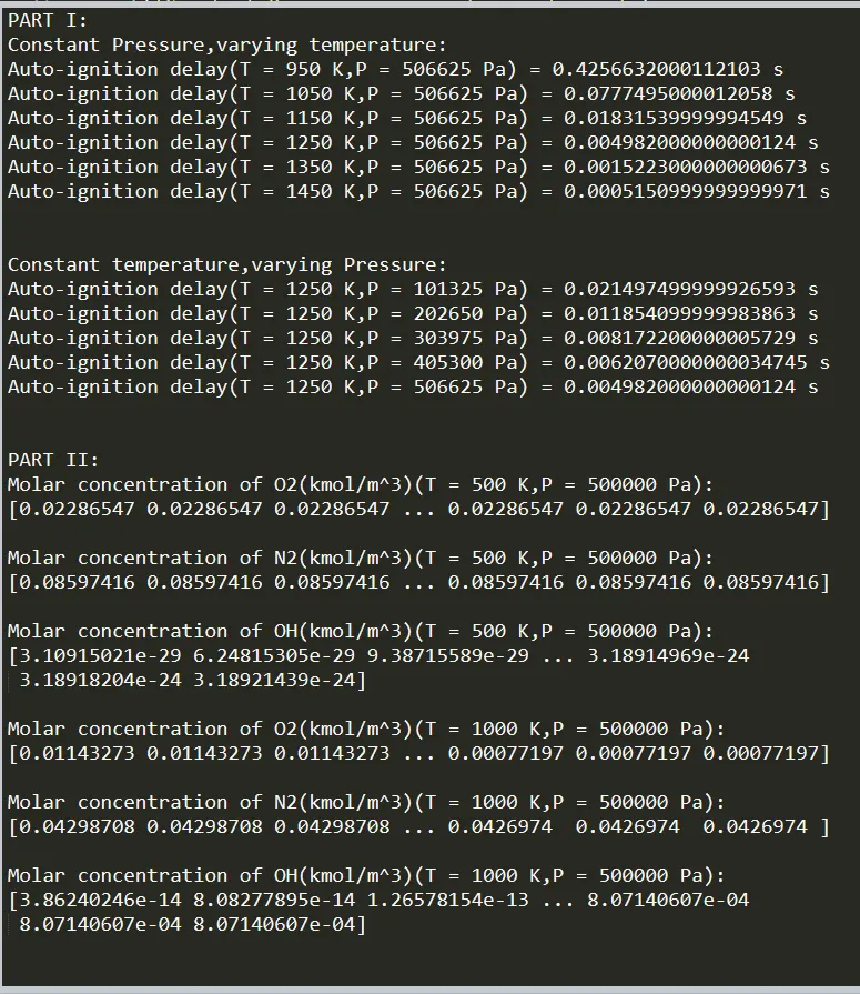
Fig(a) Results from the console window.
These results will be referenced in the sections below.
Part I:
The following plots were obtained after running the simulation.
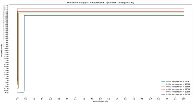
Fig(b) Simulation time vs Temperature(Constant initial pressure,varied temperature).
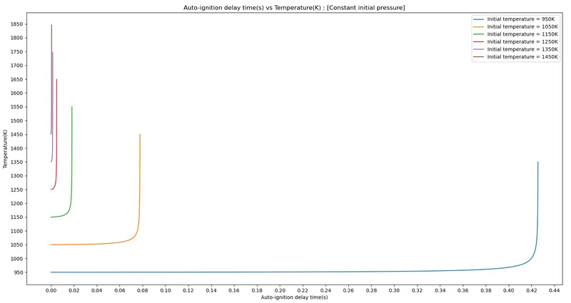
Fig(c) Auto-ignition delay time vs temperature(Constant initial pressure,varied temperature).
From the plots displayed above, a few conclusions can be made.
If the pressure of the cases are kept the same, and the initial temperature of the mixture is changed, combustion is affected significantly. In this case, the initial temperatures were increased with each run of the loop. It can be observed that the mixtures with a higher initial temperature attain significantly higher values of temperature after combustion. This can be attributed to the increase of the internal energy of the reactants. Since this is a constant-volume chamber, the temperature that is obtained from the simulation, is the adiabatic flame temperature. If the formulae for adiabatic flame temperature is observed, the difference in internal energy of the reactants and the products should be zero. But, this is usually not the case, as a small value close to zero is obtained after computation. Increasing the initial temperature of the reactants essentially causes combustion to be more adiabatic, as far as calculations are concerned. Hence, higher values of temperature are obtained, with higher initial values of temperature, while keeping the pressure constant. Of course, this effect will reduce and eventually stop at some point.
Another important observation that can be made, is the effect of the higher initial temperature on auto-ignition delay time. Auto-ignition is basically a spontaneous combustion process that takes place when the fuel reaches a certain temperature, without any external heat inducement. At lower initial temperatures, the time taken for the mixture to reach the auto-ignition temperature is considerably longer, compared to the cases with a higher initial temperature. The auto-ignition temperature in this case is taken as 400 Kelvin higher than the initial temperature of the mixture. The initial pressure plays a vital role in this case. Keeping the initial temperature constant, and increasing the temperature, promotes faster combustion of the mixture, or in this case, auto-ignition. The actual auto-ignition delay times can be seen in the console window shown above.
The degree to which pressure affects the mixture can be seen in the plots below.
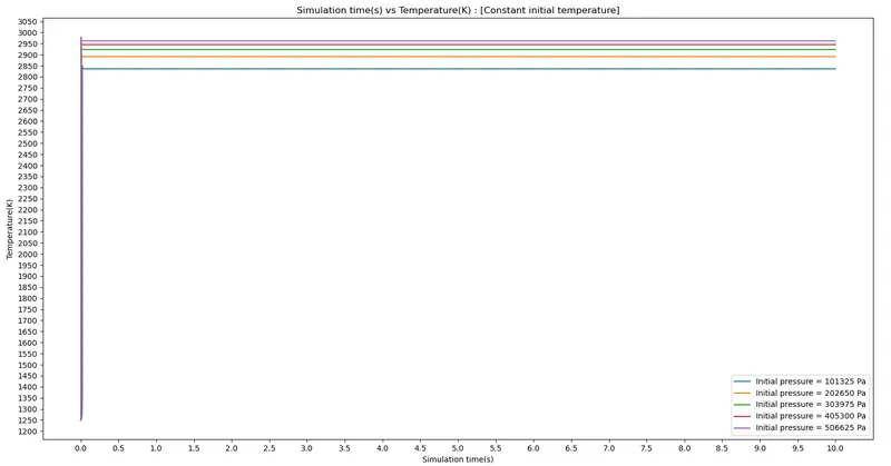
Fig(d) Simulation time vs Temperature(Constant initial temperature).
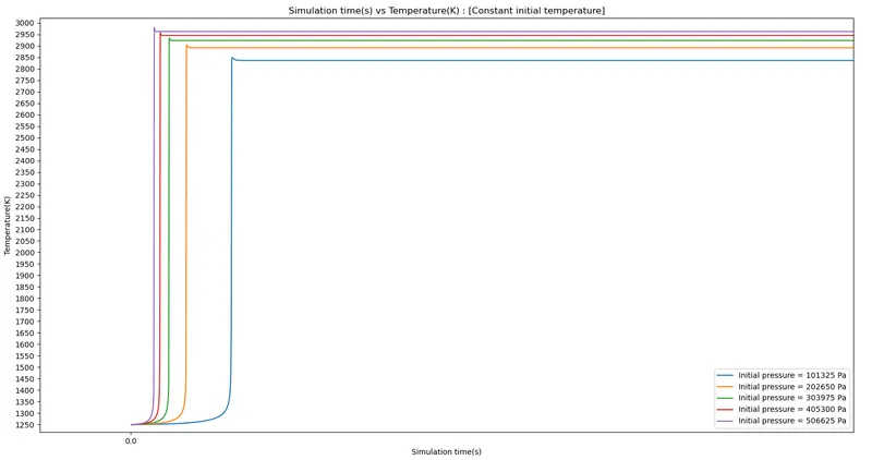
Fig(d.i): Simulation time vs Temperature(Constant initial temperature,varied pressure)[View near the initial time step]
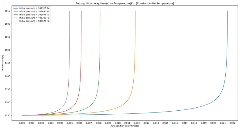
Fig(e) Auto-ignition delay time vs temperature(Constant initial temperature,varied pressure).
From the plots shown above, two conclusions can be made.
The temperature obtained after combustion is significantly higher in cases that have a higher initial pressure, despite keeping the initial temperatures the same. To put this in perspective, the working of a diesel engine can be referenced. The fuel intake occurs when the temperature of the air within the combustion chamber is high enough for the fuel to combust. The temperature of the air is increased by increasing the pressure of the air in the cylinder, by virtue of compression. Compressing the air, increases the pressure of the air, hence increasing the temperature of the air. Similarly, in this case, the initial pressure of the mixture in the reactor is increased, but the volume of the reactor remains the same in all of the cases. This suggests that increasing the initial pressure of the mixture, will allow the fuel to combust in a shorter amount of time, as the temperature is kept the same. The science behind the phenomenon is similar. To put it simply, the air-fuel mixture enters the constant-volume reactor, with a certain pressure. The initial pressure of the mixture constrained within the chamber causes the temperature of the mixture to increase rapidly, hence resulting in combustion. Increasing the initial pressure of the mixture will hasten this process, and the temperature increase of the mixture in the chamber will be more aggressive in nature, resulting in a reduction in the auto-ignition delay time. The decreasing auto-ignition delay times can be seen in the console window shown in the first figure.
The auto-ignition delay time reduces with each consecutive increase in pressure value,while keeping the pressure values the same.
Part II:
The following plots display the simulation time vs molar concentrations of O2,H2O and OH, for temperatures of 500 K and 1000 K, with a pressure of 5 bar.
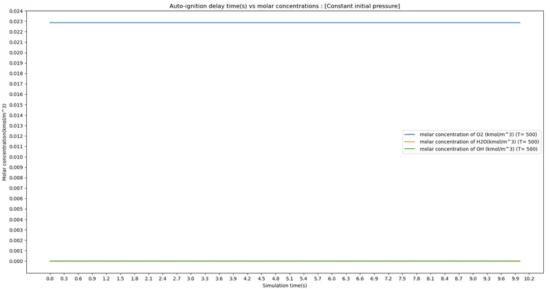
Fig(f) Simulation time vs molar concentrations(T = 500K).
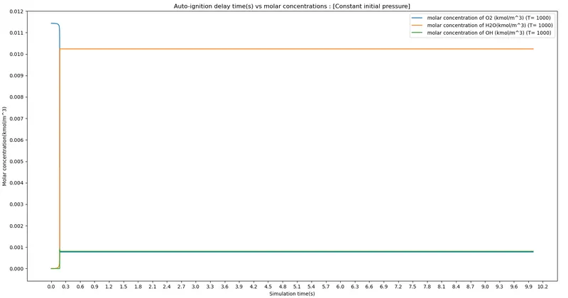
Fig(g) Simulation time vs molar concentrations(T = 1000K).
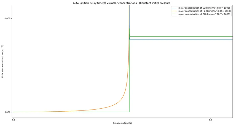
Fig(g.i) Simulation time vs molar concentrations(T = 1000K)[view near the initial time step].
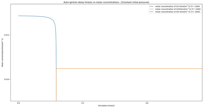
Fig(g.ii) Simulation time vs molar concentrations(T = 1000K)[view near the initial time step].
At T = 500 K, it can be observed that there is no change in the molar concentrations of the three species. Hydroxide and water have a molar concentration of around zero throughout the duration of the simulation, and this can only mean one thing. The molar concentration of these species have not increased significantly due to the fact that combustion has not taken place, as an initial temperature of 500 Kelvin and an initial pressure of 5 bar seems to be insufficient and does not meet the criteria required for auto-ignition.
However, at T = 1000K, changes in the molar concentration can be observed over a period of ten seconds. The molar concentration of oxygen is the highest during the beginning, and then drops dramatically within a small period of time. The concentrations of hydroxide and water increase dramatically. This suggests that auto-ignition has taken place. The molar concentration of water seems to be the highest after the auto-ignition delay time, and this is because the mixture is stoichiometric in nature. Water is a main product of combustion, and obtaining a large concentration of it after combustion, is logical. Since the mixture is stoichiometric, the hydroxide formation is not dramatic, and is a minor product of combustion. The reason the sudden increase of hydroxide seems unnatural in the plot, can be attributed to the fact that it is a minor product. The majority of the oxygen produces water after combustion, and the smooth increase over a curve can be observed in the plots. It is interesting to observe the molar concentration of oxygen reduce to such an extent, its concentration dips below the concentration of hydroxide, as it has been consumed during combustion, and other major and minor products contain oxygen.
Another observation that can be made, is the similarity of the behaviour of water in the plot, and the temperature increase after auto-ignition delay time shown in the previous part. Hence,a superficial conclusion that can be made is that water,after auto-ignition, has a high value of enthalpy, and contributes greatly to the temperature increase after combustion. These trends can be observed in the plots shown above.