Simulating fluid flow in an Exhaust manifold using ANSYS Fluent.

Project title : Simulating fluid flow in an exhaust manifold using ANSYS Fluent

Aim: Observing the thermal behaviour of a hot fluid flowing through the exhaust pipe, and obtaining an accurate value of the Heat Transfer Coefficient on the internal solid surface of the exhaust manifold.

Introduction:

Conjugate Heat Transfer analysis is used to capture accurate heat transfer behaviour due to both convection and conduction, for cases in which a solid and fluid at different temperatures or subjected to different thermal conditions interact with each other. This is especially useful at the fluid-solid interface, where the fluid interacts thermally with solid. The result obtained is a coupled solution, taking into account the thermal effects due to both, conduction and convection. It is also known for its flexibility, and its ability to handle complex simulations. Conjugate Heat Transfer can be used in a wide range of cases that involve mass-flow of a fluid over or inside a solid, subjected to different thermal conditions. Examples of the usage of CHT is seen in the determination of the effectiveness of heat transfer of a solid fin with a fluid flowing around it, fluid flowing through a tube at different temperature, such as a heat exchanger, and many more applications.A point to note is that CHT is not limited to just conduction and convection, but can take into consideration radiation heat transfer as well.

In this particular case, the hot fluid flowing through the exhaust pipe is air, at 450 degrees Celsius. The hot fluid interacts with the solid surface of the pipe, which is at a lower temperature, and the heat transfer at this point is due to convection. The inner wall in contact with the fluid increases in temperature, and the heat then flows from the inner wall to the outer wall. The pipe thickness is heated, caused by heat transfer due to conduction. The outer wall of the exhaust pipe is subjected to convection at 20 w/m^2, at 25 degrees Celsius.

Theory:

The exhaust manifold is a vital component in automotive design of a vehicle, as it is used to collect the exhaust gases formed due to combustion of the fuel and air within the cylinders, and provide a path for the gases to escape to the atmosphere. The exhaust manifold has multiple inlets connected to the exhaust ports on the cylinders in the engine. The high pressure exhaust gases flow through the pipe with relative ease, as the pressure difference between the exhaust pipe outlet at atmospheric pressure and the high pressure exhaust gases in the cylinder, is enough for the gases to get sucked out of the combustion chamber.

Simulation process :

The following points display the process followed in order to simulate fluid flow through the exhaust manifold. The modelling approach will be discussed in the mesh detail section and the solver type shall be discussed in the Fluent set-up section.

1) Geometry creation:

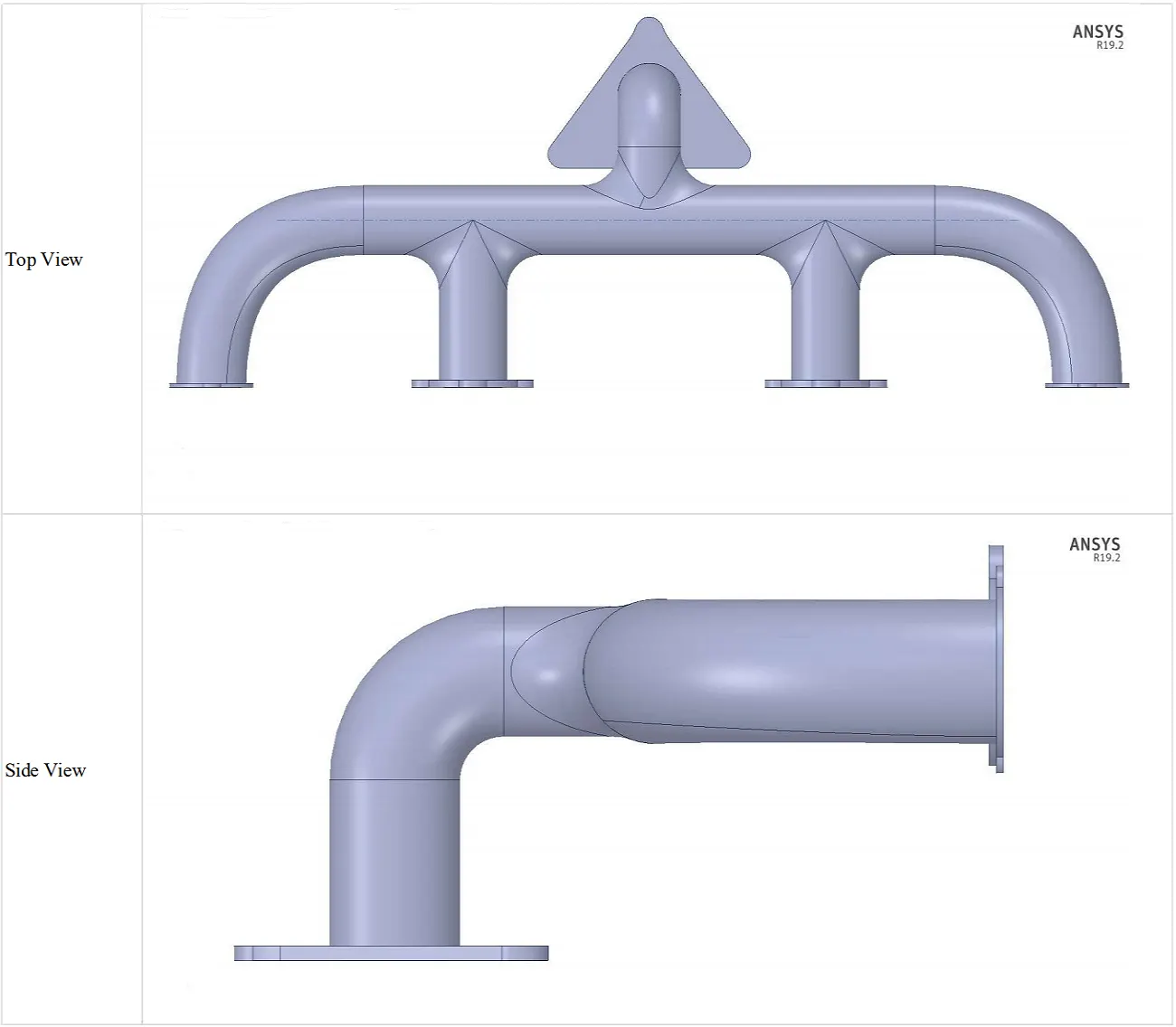
• The exhaust manifold geometry was created using SpaceClaim.
• In order to insert the fluid volume into the pipe geometry, the option 'Volume extract' under the 'Prepare' option has been used (Prepare>Volume Extract). The edges of the inlets and the outlet were selected and the volume was created within these boundaries.
• At this point, if the mesh were to be created, we would obtain a non-conformal mesh, which causes the solid and fluid surfaces to not be attached at some points. This will yield incorrect simulation results, and hence the mesh at the fluid-solid interface should share the same mesh configuration and remain attached at all points.
• Due to this reason, the topology of the two domains are shared by using the 'Share' option under 'Workbench' (Workbench>Share). This forces the fluid and solid surfaces to remain continuous and in contact at all times, at the fluid sold interface.

2) Mesh details:

Modelling approach:

• For this simulation, the accuracy of the heat transfer across the fluid-solid interface (inner wall of the exhaust manifold) is of prime importance, and hence, this area must possess higher mesh refinement compared to the other regions. This reason behind this is due to the fact that this region is affected by both conduction heat transfer in the solid, and convection heat transfer in the fluid. Since the topology of the inner wall of the solid, and the fluid in contact with the solid have been shared, the mesh refinement will be consistent between the two. The Heat Transfer Coeffcient value is calculated by taking the area average of the heat transfer coefficient values at different points on the inner wall of the exhaust manfold. Hence, a mesh of a smaller element size would prove to be better from an accuracy standpoint. Since the inner wall of the solid and the outermost layer of the fluid share the same topology, the mesh refinement for both will be the same.
• The velocity boundary layer and thermal boundary layer of the fluid near the soild boundary need to be simulated accurately, as the accuracy of heat transfer by convection is dependent on these two factors, and a normal mesh will not be able to simulate this behaviour. The mesh at this point must be in the form of layers, as the fluid in this region behaves in this manner. The laminar sublayer, buffer region and the log-law region of the boundary layer flow must be resolved with precision, and for this particular case, the log-law region is not sufficient to obtain proper heat transfer behaviour at the interface. The temperature of the fluid near the wall is different to the value of the fluid flowing along the center of the pipe, and this phenomenon is important to simulate.
• The outer wall of the exhaust manifold experiences convection by air at 25 degrees Celcius(set by boundary condition), and the thermal behaviour in this region is relatively simple. Hence, the mesh used for the exhaust manifold (except for the inner face), can be left relatively coarse.
• The fluid domain should be refined slightly more compared to the solid domain, as the behaviour of the fluid needs to be simulated accurately through the curves in the exhaust manifold.

Mesh configuration:

The following image displays the mesh configuration according to the modelling approach detailed above.

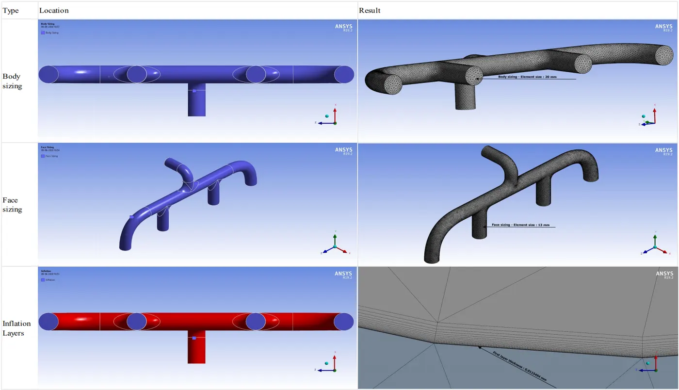
(I) Body Sizing :

• Body sizing has been utilized on the fluid body, and given an element size of 20mm.
• The mesh size of the fluid has a higher refinement compared to the solid, as the many curves in the geometry require a higher level of precision, and has been done to simulate the fluid behaviour more accurately.

(II) Face sizing:

• Face sizing has been utilized on the outermost layer of the fluid,and given an element size of 13 mm.
• As mentioned in the modelling approach section, the mesh size at the fluid-solid interface requires higher accuracy, as the Heat Transfer Coefficient uses the area average of the heat transfer coefficients at different areas of the inner wall of the exhaust manifold. The shared topology between the inner wall of the manifold and the outermost layer of the fluid forces them to have the same level of refinement.

(III) Inflation layers:

• Y-plus value selection: The laminar sublayer region of the boundary layer lies under a Y-plus value of under 5 ( Y+ < 5). The Y-plus value taken for this simulation is 0.1, and the first layer thickness of the fluid near the wall is 0.0115494mm. This ensures that the Y-plus value is under 5, and the heat transfer behaviour remains stable throughout the wall.
• The ideal range of inflation layers that should be taken is around 12 to 20, so for this simulation, 18 inflation layers have been used, with a growth rate of 1.2.

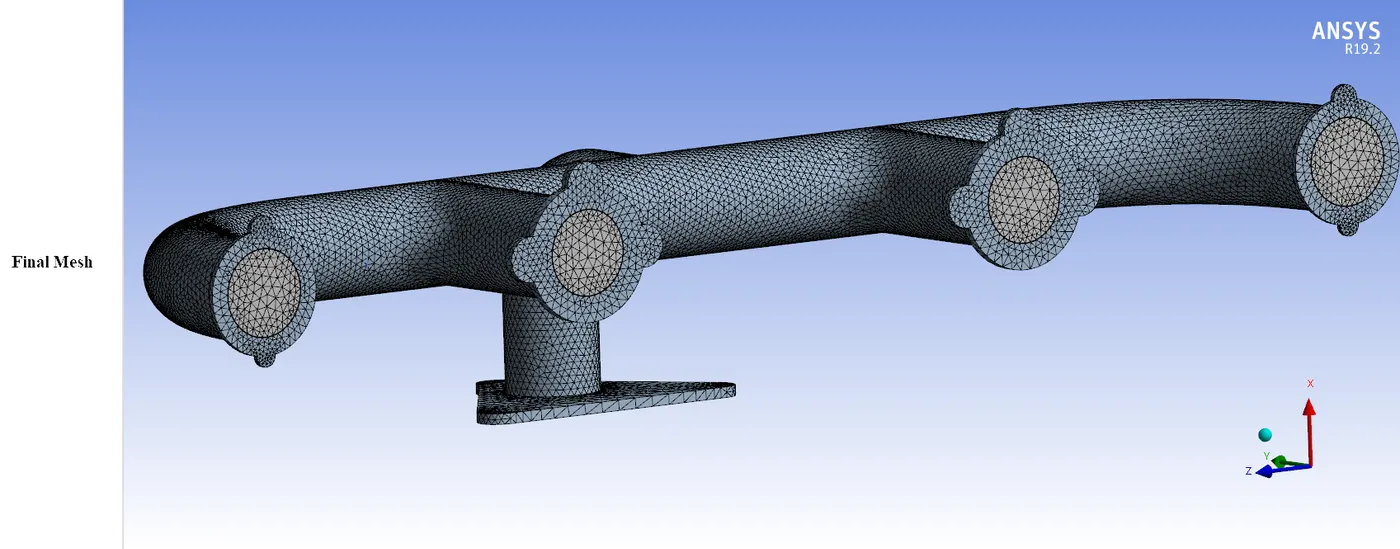
The final mesh used for the simulation is displayed in the image below.

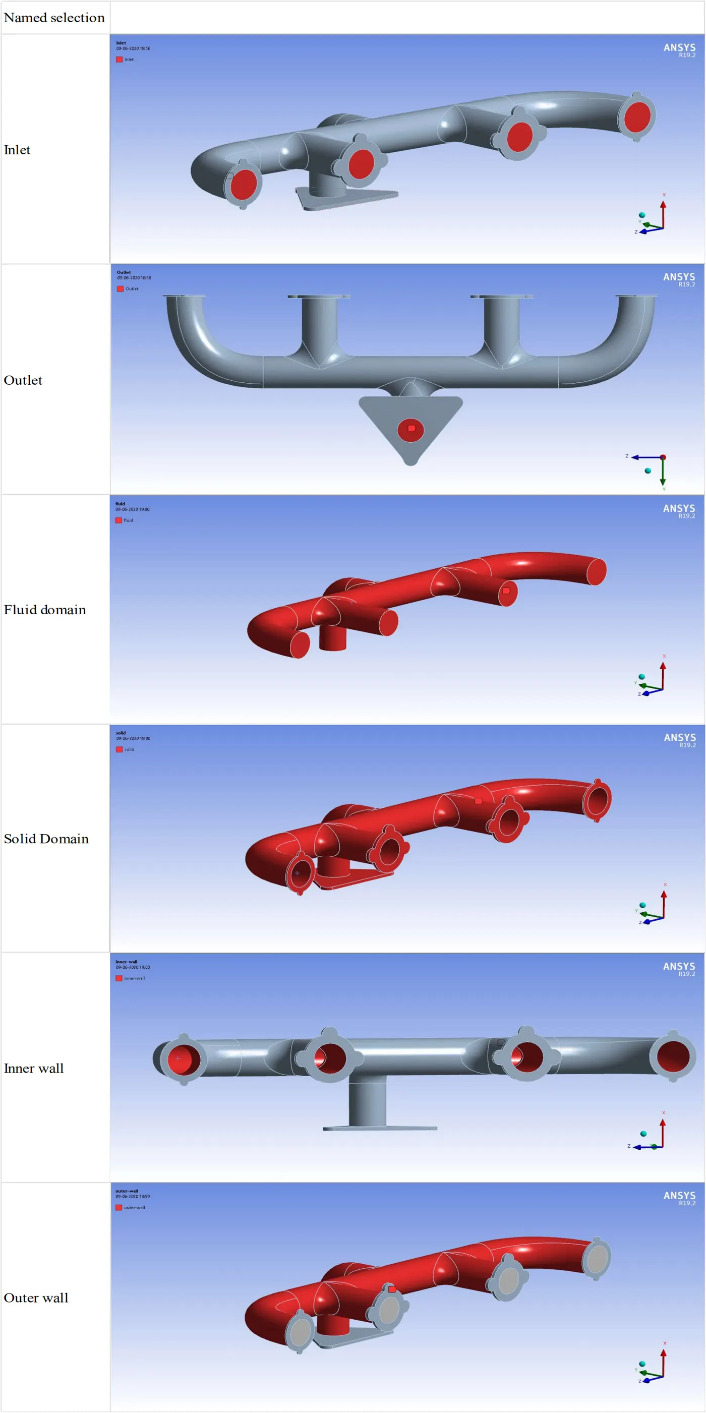
The following image displays the named selections in the mesh.

3) Fluent set-up:

Solver setting:

• Pressure-based solver

A pressure-based solver is used for this case as the mach number is under 0.3, and the compressibility effects are negligible in the flow. A density-based solver is highly accurate, but requires more computation time, and would not prove advantageous in this case. A pressure-based solver requires less computational time, and will provide accurate simulation results for this case.

Model used:

• k-omega SST

Explanation :

• The k-omega SST model has been designed to combine the advantages of the k-epsilon and k-omega turbulence models. The k-omega model solves the near-wall functions accurately, but is inaccurate in the freestream velocity sections of the fluid flow, whereas the k-epsilon model accurately solves the freestream section of the fluid flow, but provides inaccurate values at the near wall or viscous sub-layer section.
• The k-omega SST model uses a k-epsilon model in the freestream sections of the fluid flow, and a k-omega model for near-wall computations. The ability of the k-omega SST model to resolve near-wall behaviour is imperative to attaining precise thermal behaviour near the inner wall.
• This seamless switching between models is done by the integration of two blending functions 'F1' and 'F2' in the equations of specific dissipation rate and kinematic eddy viscosity respectively.
• If the value of F1 is zero, the model switches to the k-epsilon model. Similarly, if the value of F1 is one, the k-omega model is used.
• F2 involves the use of a viscosity limiter, which prevents the model from over-predicting the wall shear stress, and functions similar to F1.

Pre-processing in Fluent:

• The solver type and the steady state simulation options are set by going to Setup>General.
• The energy equation is turned on, as it is required in order to simulate heat transfer. This is done by going to Setup> Models > Energy Equation.
• The turbulence model is switched to k-omega SST by going to Setup> Models > Viscous, for the reasons stated above.
• The default fluid in fluent for the fluid is air, so no changes will be made to the material. However, this can be changed by selecting the fluid in Setup>Materials>Fluid, and then changing it in Setup>Cell Zone conditions>Fluid.

• Boundary conditions:

• The freestream velocity is set to 5 m/s at the inlet by going into Setup > Boundary Conditions > Inlet.The temperature of the fluid is changed in the same window by going to the Thermal settings in the same window, and is set to 450 degrees Celsius.
• The thermal boundary conditions of the inner wall is set to coupled.
• The thermal boundary conditions of the outer wall are changed to convection, with the heat transfer coeffcient of air set to 20 W/m^2-K and the freestream temperature of air set to 25 degrees Celcius.
• The boundary conditions of the simulation are under the same section under 'Type', and can be changed by using the dropdown provided below in the section.
• The boundary conditions are set in Fluent, as shown in the table below.

• Inlet	Velocity-inlet
  Outlet	Pressure-inlet
  Inner wall	wall
  Outer wall	wall
  Solid	interior
  Fluid	interior

• The number of iterations is set to 1000 by entering the value within the Run calculation section.

Post-processing:

• The Surface Heat Transfer coefficient contours can be obtained by entering Results > Graphics > Wall Fluxes>Surface Heat Transfer Coefficient, selecting the desired surface(in this case, the inner wall), and plotting the contour.
• The bulk temperature of the fluid at the outlet is calculated by going to Results>Reports>Surface integrals, changing the report type to Mass-weighted average, changing the field variable to Temperature, and selecting the Outlet under 'Surfaces'.
• The reference values for the Surface Heat Transfer Coefficient are provided by entering Setup > Reference values, where the surface area of the inner wall (A = 2.32 m) is entered. The velocity is set as 5 m/s, and the reference temperature is set by entering the bulk temperature of the fluid at the outlet. This will be elaborated upon in the Result section.
• The Surface Heat Transfer Coeffcient is calculated by going to Results>Reports>Surface integrals, changing the report type to area-average, changing the field variable to Wall Fluxes>Surface Heat Transfer Coefficient, and selecting the inner wall, under 'Surfaces'.

Results:

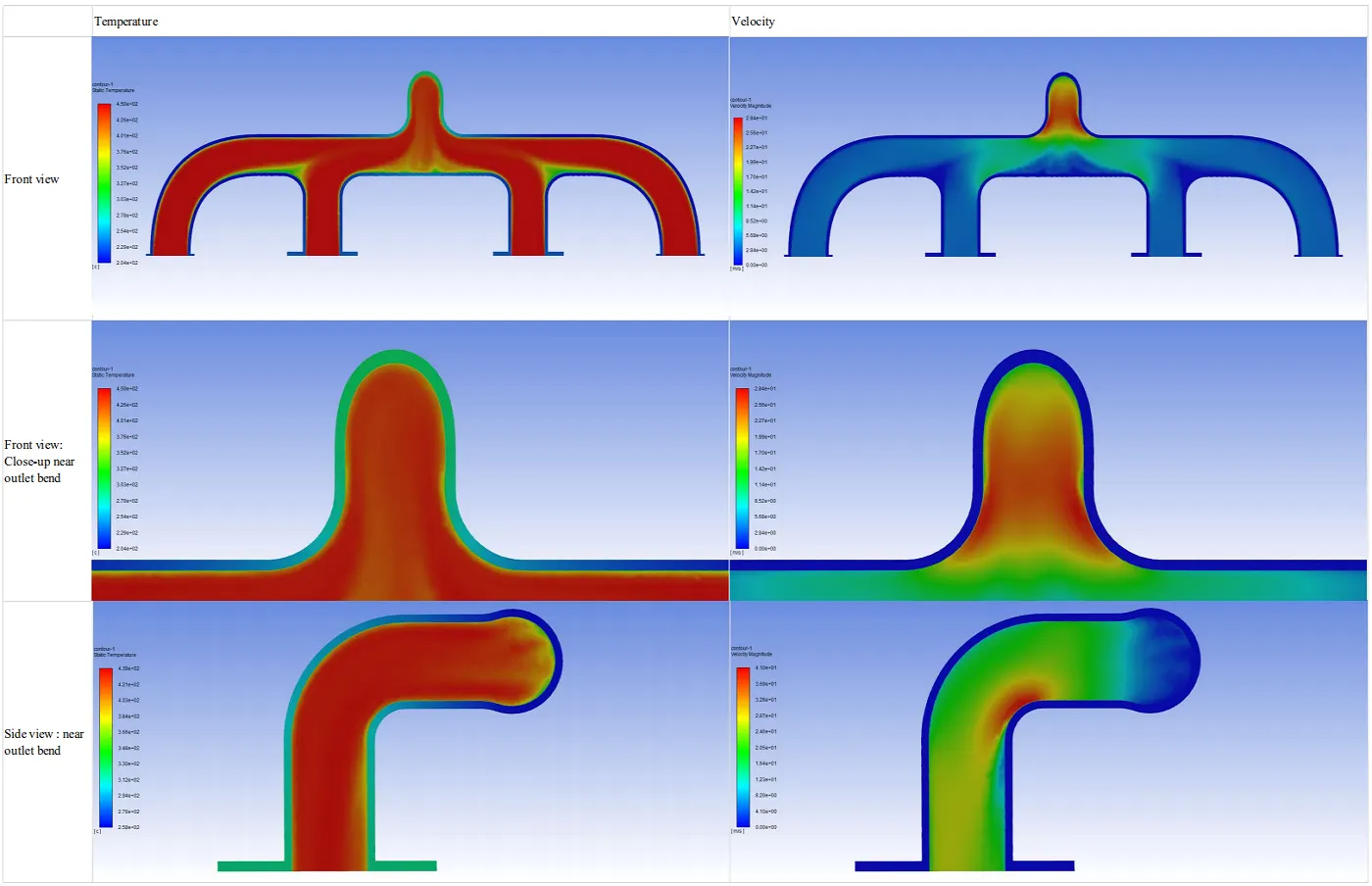
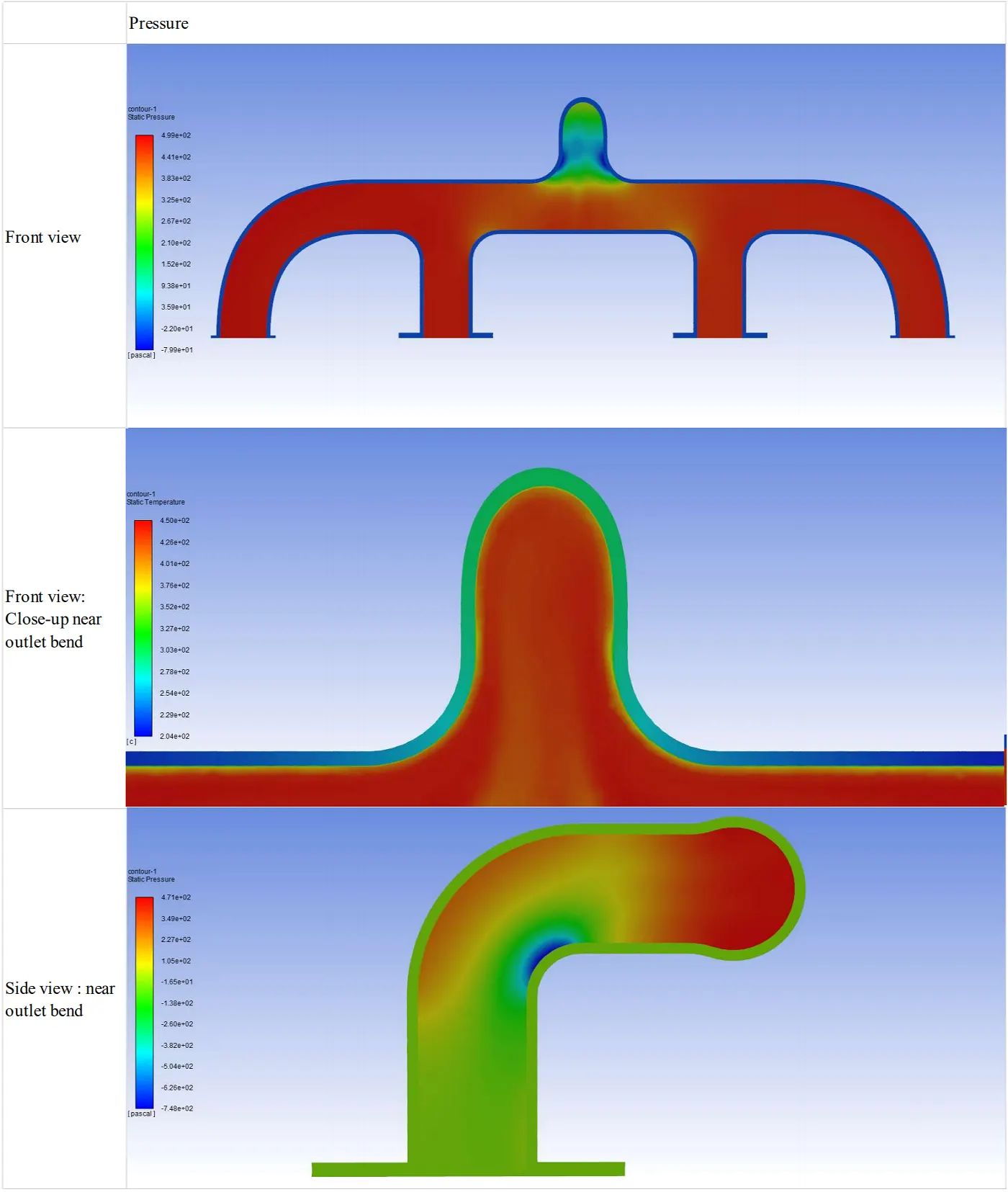
The temperature,pressure and velocity contours for the front and side views of a plane.

Explanation:

• From the contour plots above, a couple of inferences can be made. The main inference that can be drawn, is from the relation between the temperature of the wall and the velocity of the fluid. However, understanding this requires understanding the behaviour of the fluid in terms of pressure and velocity as a prerequisite.
• There are three areas where pressure drop is observed; near the two exit bends of the two inlets closest to the outlet, the two bends at the entrance to the single outlet, and the final bend before the outlet.
• The fluid flow from the left pair of inlets and the right pair of inlets oppose each other, creating a region with increased pressure, due to fluid collision before the entrance of the outlet. It should be noted that this pressure is not as high as the pressure of the fluid near the two inlet entrance regions of the inlets between the two outermost inlets, as there is a small but significant pressure drop near their respective exit bends. This can be due to the formation of favourable pressure gradients in those regions, possibly due to the sudden bend in the geometry, causing an increase in velocity. But, as mentioned above, the collision of the two opposing fluid flows causes an increase in pressure again just before the entrance of the outlet, and exerts a force on the fluid that is moving over this region. This increases the velocity over the entrance bends of the outlet, hence causing a signifcant drop in pressure. Once again, favourable pressure gradients on the bends near the entrance of the outlet are created, but the pressure drop in these regions are significantly higher than those of the previously mentioned regions.
• Another pressure drop is observed at the final bend, caused due to the reasons that have been expained above. But there are two differences, the first being, that in this case, that the velocity is already significantly high, so the pressure drop at the final bend is the highest, and the velocity is the highest in this region and the second difference being, the pressure on the outer bend of the final bend is high, so it contributes to the increased velocity of the fluid around the inner bend by exerting a force on it.
• If the heat transfer behaviour is seen at the wall, elevated temperatures can be observed around the exit bend of the exhaust manifold.
• The heat transfer is directly related to the velocity of the fluid. The temperature of the solid wall is higher compared to the rest of the body, if the high velocity zones are observed. Hence, it can be said that the high velocity of the fluid induces high heat transfer at the boundary. This behaviour can be observed more clearly by using the surface heat transfer coefficient and heat flux contour.

Surface Heat Transfer Coeffcient:

The following image displays the surface heat transfer coefficient and heat flux contours of the inner wall.

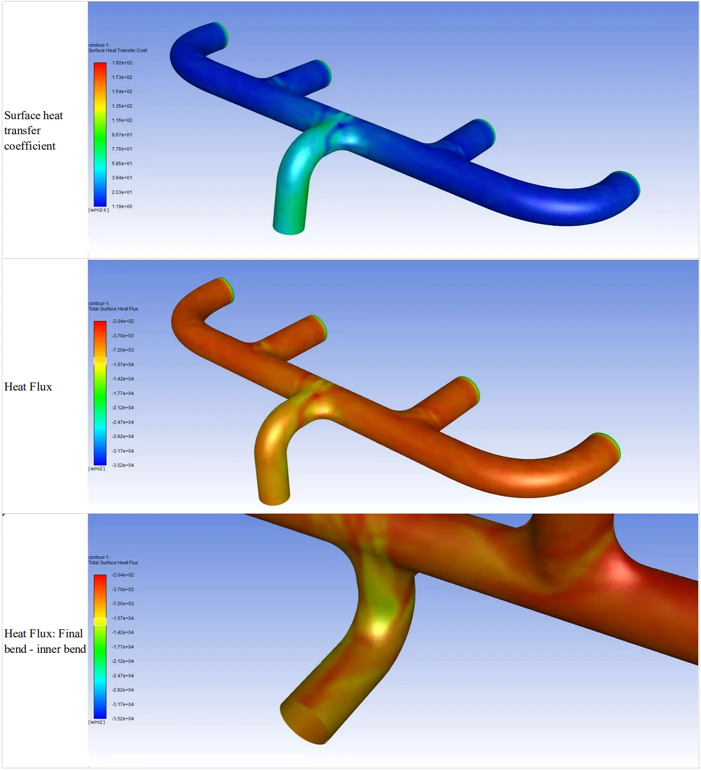
• It can be observed that the surface heat transfer coefficient is relatively higher along the outlet pipe surface. This proves that the assumption that the high velocity of the fluid within the domain in this section promotes heat transfer across the walls, and is the reason for the higher temperature in the solid wall.
• However, if the value of velocity is high in a very small region, it would not have much of an effect on the temperature of the wall. But,as we can see in the images displayed above, the high velocity region dominates the outlet, and hence, the heat transfer coefficient of the inner wall is directly influenced by it, causing increased heat transfer values in near the outlet region, whereas the low velocity regions have much lower heat transfer coefficient values.
• At the final bend, if we look at the region where the velocity is supposed to be the maximum, the heat flux in that region seems to be the highest. Hence, it can be concluded that the heat transfer due to convection is significantly higher than the regions surrounding it, as the velocity is the highest near this surface.

Reliability of surface heat transfer coefficient results obtained from fluent:

The following relation is used by fluid to compute the surface heat transfer coefficient:

h = q/[T(wall) - T(bulk)]

where,

h = heat transfer coefficient

q = heat flux (W/m^2)

T(wall) = wall temperature(K)

T(bulk) = bulk temperature(K)

• The surface heat transfer coefficient in Fluent is highly sensitive to the reference temperature that has been set in the 'Reference values', section. The reference temperature taken into consideration by Fluent is the bulk temperature of the fluid. The bulk temperature plays an important role in the computation of the surface heat transfer coefficient, and must be set accurately in order to obtain accurate results. However, the bulk temperature of the fluid is a static value, and does not change with respect to each section of the pipe.
• This key factor is the main disadvantage of the values of the surface heat transfer coefficient obtained from the simulation. This value would hold for a simple geometry, but for a complex geometry, this may not yield the same levels of accuracy.
• The bulk temperature of the fluid is the mass-weighted average of temperature at a particular section. The values of bulk temperature change at different sections of the pipe. For this particular simulation, the bulk temperature has been calculated for the entire fluid domain by taking the mass-weighted average of the entire fluid domain, as it will be a value that is fair during calculations at all regions of the inner wall.
• In this case, the bulk temperature is 435 degrees Celcius. Using this value as a reference, the average surface heat transfer coefficient of the inner wall comes to 26.47061 W/m^2-K.

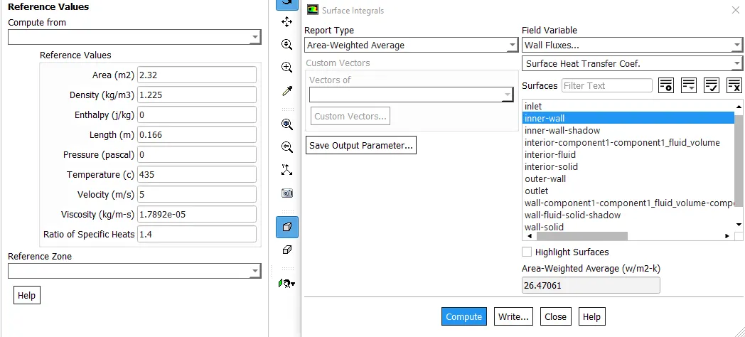
• The only possible way to validate this result is to use some form of emperical relation, which will give us an estimate of the heat transfer coefficient value that should be obtained from the simulation, if this cannot be verified experimentally.
• The Dittus-Boelter equation for the Nusselt number has been used to find the Nusselt number of the pipe, and then this value is used to attain the surface heat transfer coefficient.
• The following emperical relation has been used to attain the Nusselt number, and the equation below it has been used to calculate the heat transfer coefficient at the inner wall.

Nu = `0.023*Re^(0.8)*Pr^(0.3)`

where,

Re = Reynolds number = `(rho*v*d)/mu`= (1.225*5*0.166)/(1.7892)

Pr = Prandtl Number = `(Cp*mu)/k` = (1006.43*1.7892*10^(-5))/(0.0242)

`Cp` = specific heat of air

`rho` = density of air

`mu` = dynamic viscocity

k = thermal conductivity of air

Nu = `0.023*((1.225*5*0.166)/(1.7892*10^-5))^(0.8)*((1006.43*1.7892*10^(-5))/(0.0242))^(0.3)`

Nu = 133.92

Substituting this value in the following equation,

h = `(Nu*k)/d`

h = 133.92*0.0242/0.166

where,

h = surface heat transfer coefficient

d = inner diameter

h = 19.5239 W/m^2-K

Upon solving the equation, we get a value of 19.5239 W/m^2-K.

• The value that has been obtained by this emperical relation is around the value that has been obtained by the simulation. This emperical relation is a primitive relation, and does not take into account the complexities of the pipe, or the various regions of increased velocity and pressure drop. But, this equation gives us a value around which the value of the heat transfer coefficient should lie.
• Hence, we can say that the value obtained by simulation is more or less accurate.

Another factor that this value depends on is the quality of the mesh. A lower mesh quality will yield relatively innacurate results, and to calculate sensitive values such as the heat transfer coefficient,or rather, for heat transfer problems in general, the mesh should be fine. Due to the limitations on the mesh, the highest level of accuracy might not have been achieved, but it is sufficient to display the heat transfer behaviour at the fluid solid interface.

Conclusions:

The average surface heat transfer coefficient of the inner wall was found to be 26.47061 W/m^2-K. The surface heat transfer coefficient values achieved by simulation are highly sensitive to the reference temperature, a temperature that is set as a post-processed value. If possible, the surface heat transfer coefficient should not be relied upon as a quantity to describe the heat transfer behaviour. The main disadvantage of having a static reference value of temperature is that it does not account for the temperature at each and every section of the pipe, and does not capture the conditions specific to a particular part of the geometry. Due to this, there is a possibility of over-predicting or under-predicting the heat transfer coeffcient values at some regions. Again, due to this reason, relying on the heat transfer coefficient to accurately capture the heat transfer behaviour at a certain wall would not be advisable.

If a reliable quantity is required to observe the heat transfer at the wall, the heat flux should be utilized. The heat flux is a product of the simulation, and will have a higher degree of accuracy, as it is not influenced by changing the reference temperature. It will give a more reliable as well as accurate depiction of the heat transfer on the wall compared to the surface heat transfer coeffficient. The surface heat transfer coefficient does use the heat flux values in its equation, but the advantage of having the accuracy of the heat flux values is lost due to the use of the static reference temperature value.