Week 7 - Simulation of a 1D Super-sonic nozzle flow simulation using Macormack Method
Simulation of a 1D Super-sonic nozzle flow simulation using Macormack Method
Nozzle
A nozzle is a device designed to control the direction or characteristics of a fluid flow (specially to increase velocity) as it exits (or enters) an enclosed chamber or pipe.
A nozzle is often a pipe or tube of varying cross sectional area, and it can be used to direct or modify the flow of a fluid (liquid or gas). Nozzles are frequently used to control the rate of flow, speed, direction, mass, shape, and/or the pressure of the stream that emerges from them. In a nozzle, the velocity of fluid increases at the expense of its pressure energy.
Applications of a Nozzle:
There are following applications of a nozzle are:
1. Nozzles are used in steam turbines, gas turbines, water turbines and in jet engines, Jet propulsion.
2. Nozzles are used for flow measurement e.g. in venturimeter.
3. Nozzles are used to remove air from a condenser.
4. Injectors for pumping feed water to boilers.
5. Artificial fountains.
There are three types of nozzles:
1. Convergent nozzle,
2. Divergent nozzle, and
3. Convergent-Divergent nozzle.
If the cross-section of the nozzle decreases continuously from entrance to exit, it is called a convergent nozzle.
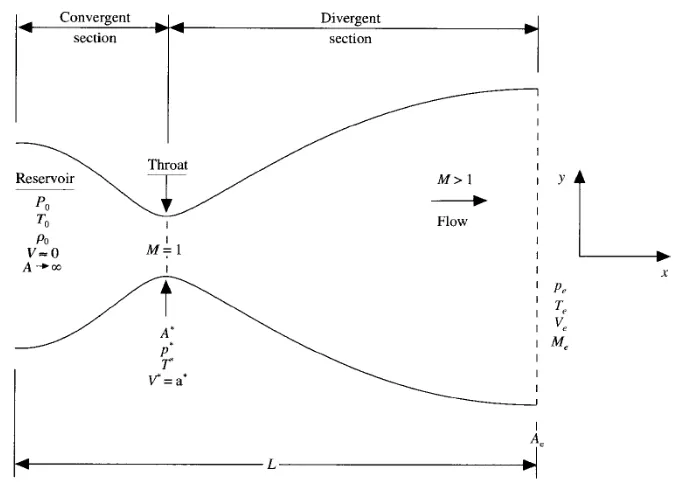
If the cross-section of the nozzle increases continuously from entrance to exit, it is called a divergent nozzle. If the cross-section of the nozzle first decreases and then increases, it is called a convergent-divergent nozzle. The section where cross-sectional area is minimum is called ‘throat’ of the nozzle.
General-Flow Analysis of a Nozzle:
Assumptions:
1. The flow of the fluid is assumed to be one dimensional.
2. The change in area and curvature along the axis of the duct are gradual.
3. Thermodynamic and mechanical properties are uniform across planes normal to the axis of a duct.
4. The flow of the fluid is assumed to be steady flow.
Schematic representation of a 1D convergent divergent nozzle
MacCormack method
In computational fluid dynamics, the MacCormack method is a widely used discretization scheme for the numerical solution of hyperbolic partial differential equations. This second-order finite difference method was introduced by Robert W. MacCormack in 1969. The MacCormack method is elegant and easy to understand and program.
The MacCormack method is a variation of the two-step Lax–Wendroff scheme but is much simpler in application. To illustrate the algorithm, consider the following first order hyperbolic equation

The application of MacCormack method to the above equation proceeds in two steps; a predictor step which is followed by a corrector step.
Predictor step: In the predictor step, a "provisional" value of u at time level n+1) is estimated as follows

The above equation is obtained by replacing the spatial and temporal derivatives in the previous first order hyperbolic equation using forward differences.
Corrector step: In the corrector step, the predicted value `u_{i}^{overline {n+1}`is corrected according to the equation

Note that the corrector step uses backward finite difference approximations for spatial derivative. The time-step used in the corrector step is `{(Delta t)/2}` in contrast to the `Delta t` used in the predictor step.
Replacing the `u_{i}^{(n+1)/2}` term by the temporal average

to obtain the corrector step as

The MacCormack method is well suited for nonlinear equations (Inviscid Burgers equation, Euler equations, etc.) The order of differencing can be reversed for the time step (i.e., forward/backward followed by backward/forward). For nonlinear equations, this procedure provides the best results. For linear equations, the MacCormack scheme is equivalent to the Lax–Wendroff method.
Unlike first-order upwind scheme, the MacCormack does not introduce diffusive errors in the solution. However, it is known to introduce dispersive errors (Gibbs phenomenon) in the region where the gradient is high.
Conservative forms
In these form of mathematical models ,the control volume is stationary.
The governing equation is given by
`del/(delt)(rhoAdx) +del(rhoAV) =0`
Dividing by dx
`del/(delt)(rhoA) +del/(delx)(rhoAV) =0`
So the continuity equation is given in the Quasi 1D form as
`del/(delt)(rhoA) +Vdel/(delx)(rhoA) =-rho A(delV)/(delx)`
Similarly the momentum and energy equations are given by
`frac{del(rhoAV)}{delt} + frac{del[rhoAV^2 + (1/gamma)pA]}{delx} = frac{1}{gamma}p(frac{delA}{delx})`
frac{del[rho(frac{e}{gamma-1} + frac{gamma}{2}V^2)A]}{delt} + frac{del[rho(frac{e}{gamma-1} + frac{gamma}{2}V^2)AV + rhoAV]}{delx} = 0
The above equations of conservative form can not be discretized directly , let the equations be described in form of solution vector U, flux terms F and source terms J .
`U_1 = rhoA`
`U_2 = rhoAV`
`U_3 = rho(frac{e}{gamma-1} + frac{gamma}{2}V^2)A`
`F_1 = rhoAV = U_2`
`F_2 = rhoAV^2 + frac{1}{gamma}rhoA`
`F_3 = rho(frac{e}{gamma-1} + frac{gamma}{2}V^2)AV + rhoAV`
`J_2 = frac{1}{gamma}rhofrac{delA}{delx}`
Substituting these values in the above equations we get
`frac{delU_1}{delt} = - frac{delF_1}{delx}`
`frac{delU_2}{delt} = - frac{delF_2}{delx} + J_2`
`frac{delU_3}{delt} = - frac{delF_3}{delx}`
On further simplification of the above terms
`F_1 = U_2`
`F_2 = frac{U_2^2}{U_1} + frac{gamma - 1}{gamma}(U_3 - frac{gamma}{2}frac{U_2^2}{U_1})`
`F_3 = gammafrac{U_2U_3}{U_1} - frac{gamma(gamma - 1)}{2}frac{U_2^3}{U_1^2}`
`J_2 = frac{1}{gamma}rhoTfrac{delA}{delx} = frac{gamma - 1}{gamma}(U_3 - frac{gamma}{2}frac{U_2^2}{U_1})frac{del(lnA)}{delx}`
Non conservative forms
In these form of mathematical models ,the control volume is moving.
In this case the continuity,momentum and energy equations are given by
`-rho'(delV')/(delx') -rho'V'del/(delx')(lnA)-V'(delrho')/(delx') =(delP')/(delt')`
`-V'(delV')/(delx') - 1/gamma((delt')/(delx')+(T')/(rho') (delrho')/(delx')) =(delV')/(delt')`
`-V'(delT')/(delx') -(gamma-1)T'[(delV')/(delx')+V'(del)/(delx')(lnA)] =(delT')/(delt')`
The steps involving in writing the code are
1. Meshing
2. Discretizing
3. Solving for the initial and boundary conditions.
Non dimensionalization of parameters
Distance `x' = x/l`
Pressure `P' = P/P_0`
Density `rho' =rho/rho_0`
Velocity `V' =V/a_0` where `a_0 = sqrt(gammarT_0)`
Time `t' = t/(L/a_0)`
Area `A' =A/(A^**)`
Initial and boundary conditions
n=31;
Non conservative form
Boundary Conditions
For Non-Conservative Form
The unsteady, inviscid flow is governed by hyperbolic equations and therefore for 1D flow there exists two characertistic lines through any point in xt plane. The direction of stream line flow is from left to right i.e. from point 1 to point N.At the subsonic point, since the local velocity is less velocity of sound hence, the left running characteristic at point 1 travels upstream against the low velocity sub sonic flow which is moving slowly from left to right. Hence, the resultant velocity of left running characteristic will be `a_1-V_1`.This left running characteristic is moving out of the domain as the domain under consideration is from point 1 to point N.
However, the right running characteristic is moving to the right at i.e into the domain. This is due to the fact that the fluid element at point 1 is already moving into the domain. Also the right running characteristic is moving to the right at velocity of `a_2-V_2`
The choice of boundary conditions will be decided using the above method of characteristics. The method of characteristics tells us that at a boundary where one characteristic flows into the domain then value of one dependent flow field variable must be specified at that boundary and if one characteristic flows out of the domain then value of one dependent flow field variable must be allowed to float at that boundary.
Also as noted above , stream line also enters the flow of domain, hence another flow field variable must be specified at the inlet boundary.
So at the inlet two values must be specified while one value of flow field variable must be allowed to float.
Applying similar logic to the super sonic point at the outlet, we observe that the left running characteristic is propagating towards the left. However, since the fluid element itself is super sonic the left running characteristic gets swept downstream relative to nozzle with a relative velocity of `V_N-a_N`.The right running characteristic also flows downstream with a relative velocity of `V_N+a_N`.
As both the characteristics are moving out of the domain at the outlet, hence no flow field variables need to be specified at the outlet boundary. All dependent flow field variables will be allowed to float.
The variable chosen to float at the sub sonic inlet is Velocity V. Hence the value at point 1 will be calculated by linear extrapolation.
Other flow field variables will be fixed and hence will be independent with respect to time.
At super sonic outflow all flow field variables are allowed to float by applying linear extrapolation.
Conservative form
Inlet : Two dependent flow field variables to be specified at boundary while one is allowed to float.
Outlet : All flow field variables are allowed to float.
Main Scripts
Non conservative approach
clear all
close all
clc

%Inputs
n=31;
x = linspace(0,3,n);
dx =x(2)-x(1);
gamma =1.4;
nt=1400;
% dt=0.01;

%Calculate initial profiles

rho = 1-0.3146*x; %density
t = 1-0.2314*x;   %Temperature
v = (0.1+1.09*x).*t.^0.5; %Velocity

a  = 1+2.2*(x-1.5).^2; %area
throat = find(a==1);
M= v./(t.^0.5);        %mach number
        %mass flow rate
p=rho.*t;                %pressure
%Courant Number
C = 0.5;

%Code structure
%time steps

%Outer time loop
for k =1:nt
    %Time-step control
    dt = min(C.*dx./(sqrt(t) + v));
    rho_old=rho;
    v_old = v;
    t_old=t;

    %Predictor step

    for j =2:n-1
        %drho_dt_p = -rho(j)*(v(j+1)-v(j))/dx -rho(j)*v(j)*(log(a(j+1))-log(a(j)))/dx-v(j)*(rho(j+1)-rho(j))/dx;
        dvdx =(v(j+1)-v(j))/dx;
        drhodx = (rho(j+1)-rho(j))/dx;
        dtdx = (t(j+1)-t(j))/dx;
        dlogadx = (log(a(j+1))-log(a(j)))/dx;

        %Continuity equation
        drhodt_p(j) = -rho(j)*dvdx -rho(j)*v(j)*dlogadx-v(j)*drhodx;

        %Momentum Equation
        dvdt_p(j) = -v(j)*dvdx -(1/gamma)*(dtdx+(t(j)/rho(j))*drhodx);

        %Energy equation
        dtdt_p(j) = -v(j)*dtdx-(gamma-1)*t(j)*(dvdx+v(j)*dlogadx);

%         %Solution update
         rho(j) =rho(j)+drhodt_p(j)*dt;
         v(j) = v(j)+dvdt_p(j)*dt;
         t(j)= t(j)+dtdt_p(j)*dt;
    end


       %Corrector method using backward differencing
       for j =2:n-1
        %drho_dt_p = -rho(j)*(v(j)-v(j-1))/dx -rho(j)*v(j)*(log(a(j))-log(a(j-1)))/dx-v(j)*(rho(j)-rho(j-1))/dx;
        dvdx =(v(j)-v(j-1))/dx;
        drhodx = (rho(j)-rho(j-1))/dx;
        dtdx = (t(j)-t(j-1))/dx;
        dlogadx = (log(a(j))-log(a(j-1)))/dx;

        %Continuity equation
        drhodt_c(j) = -rho(j)*dvdx -rho(j)*v(j)*dlogadx-v(j)*drhodx;

        %Momentum Equation
        dvdt_c(j) = -v(j)*dvdx -(1/gamma)*(dtdx+(t(j)/rho(j))*drhodx);

        %Energy equation
        dtdt_c(j) = -v(j)*dtdx-(gamma-1)*t(j)*(dvdx+v(j)*dlogadx);

         %Solution update is not required

        end
      %Compute the average time derivative

      drhodt=0.5*(drhodt_p+drhodt_c);
      dvdt=0.5*(dvdt_p+dvdt_c);
      dtdt=0.5*(dtdt_p+dtdt_c);

      %Final solution update
      for i=2:n-1
         rho(i) =rho_old(i)+drhodt(i)*dt;
         v(i) = v_old(i)+dvdt(i)*dt;
         t(i)= t_old(i)+dtdt(i)*dt;
      end

      %Apply boundary conditions
      %Inlet
      v(1) = 2*v(2)-v(3);

      %Outlet
      rho(n)= 2*rho(n-1)-rho(n-2);
      v(n)= 2*v(n-1)-v(n-2);
      t(n)= 2*t(n-1)-t(n-2);

      m = rho.*a.*v;
     %Calculating Variables at throat section
    rho_th(k) =  rho(throat);
    t_th(k) =    t(throat);
    v_th(k) =   v(throat);
    m_th(k) =   m(throat);
    P_th(k) =   p(throat);
    M_th(k) =    M(throat);

      %Plotting for various time steps
      hold on
      figure(2)
      if k == 1
      plot(x,m)

      elseif k == 50
      plot(x,m)

      elseif k == 100
      plot(x,m)

      elseif k == 840
      plot(x,m)

      elseif k == 1400
      plot(x,m)
      end
end
      grid on
      xlabel('Nozzle length')
      ylabel('Mass flow rate')
      title('Plot for nozzle length vs mass flow rate at various time steps')
      pause(0.3)

      title_text = sprintf('Time step=%d',k);

figure(1)

     subplot(5,1,1)
     plot(x,v,'b')
     xlabel('Nozzle length')
     ylabel('Velocity')
     title('Steady-state distribution of primitive variables inside the nozzle Non-Conservative form')
     subplot(5,1,2)
     plot(x,p,'r')
     xlabel('Nozzle length')
     ylabel('Pressure')
     subplot(5,1,3)
     plot(x,t,'k')
     xlabel('Nozzle length')
     ylabel('Temperature')
     subplot(5,1,4)
     plot(x,rho,'m')
     xlabel('Nozzle length')
     ylabel('Density')
     subplot(5,1,5)
     plot(x,M,'g')
     xlabel('Nozzle length')
     ylabel('Mach number')
     ylim([-0.1 3.7])

     grid on

     %Timestep variation of properties at throat area in Non Conservative form
figure(3)

%Density
subplot(6,1,1)
plot(linspace(1,nt,nt),rho_th,'color','m')
ylabel('Density')
legend({'Density at throat'});
axis([0 1400 0 1.3]);
grid minor;
title('Timestep variation at throat area - NON CONSERVATIVE FORM')

%Temperature
subplot(6,1,2)
plot(linspace(1,nt,nt),t_th,'color','r')
ylabel('Temperature')
legend({'Temperature at throat'});
axis([0 1400 0.6 1]);
grid minor;

%Pressure
subplot(6,1,3)
plot(linspace(1,nt,nt),P_th,'color','g')
ylabel('Pressure')
legend({'Pressure at throat'});
axis([0 1400 0.3 0.5]);
grid minor

%Mach Number
subplot(6,1,4)
plot(linspace(1,nt,nt),M_th,'color','y')
xlabel('Timesteps')
ylabel('Mach Number')
legend({'Mach Number at throat'});
axis([0 1400 1 2]);
grid minor
%Mass flow rate
subplot(6,1,5)
plot(linspace(1,nt,nt),m_th,'color','k')
xlabel('Timesteps')
ylabel('Mass flow rate')
legend({'Mass flow rate at throat'});
axis([0 1400 0.5 1.1]);
grid minor
%Velocity
subplot(6,1,6)
plot(linspace(1,nt,nt),v_th,'color','b')
xlabel('Timesteps')
ylabel('Velocity')
legend({'Velocity at throat'});
axis([0 1400 0.6 1.4]);
grid minor
Conservative approach
clear all
close all
clc

%Inputs
n=31;
x = linspace(0,3,n);
dx =x(2)-x(1);
gamma =1.4;
nt=1400;

%Calculate initial profiles
for s=1:length(x)
    if (x(s)<=0.5)
        rho(s) = 1;
        t(s) = 1;
    elseif (x(s)>0.5) && (x(s)<=1.5)
        rho(s) = 1-0.366*(x(s)-0.5);
        t(s)= 1-0.167*(x(s)-0.5);
    elseif (x(s)>1.5) && (x(s)<=3.5)
        rho(s) = 0.634-0.3879*(x(s)-1.5);
        t(s)= 0.833-0.3507*(x(s)-1.5);
    end
end

a  = 1+2.2*(x-1.5).^2; %area
throat = find(a==1);
%Initialization of solution variables
u1 = rho.*a;
u2 = 0.59*ones(1,n); % this is done to calculate velocity
v =u2/u1;
u3 = u1.*(t./(gamma-1)+(gamma/2).*v.^2);
M= v./(t.^0.5);        %mach number
m = rho.*a.*v;         %mass flow rate
p=rho.*t;   %pressure
%Courant Number
C = 0.5;
%Code structure
%time steps

%Outer time loop
for k =1:nt
    dt = min(C.*dx./(sqrt(t) + v));
    u1_old=u1;
    u2_old = u2;
    u3_old=u3;

    %Predictor step
    %Initialization flux
    for j =2:n-1
        f1=u2;
        f2 = ((u2.^2)./u1) + (((gamma-1)/gamma)*(u3-(gamma/2)*((u2.^2)./u1)));
        f3 = (gamma*(u2.*u3)./u1) - ((gamma*(gamma-1)/2)*((u2.^3)./(u1.^2)));
        %Source term
        j_p = (1/gamma)*rho(j)*t(j)*((a(j+1)-a(j))/dx);
        %Continuity equation
        du1dt_p(j) = -(f1(j+1)-f1(j))./dx;

        %Momentum Equation
        du2dt_p(j) = -(f2(j+1)-f2(j))./dx +j_p;

        %Energy equation
        du3dt_p(j) = -(f3(j+1)-f3(j))./dx;

         %Solution update
         u1(j) =u1_old(j)+du1dt_p(j)*dt;
         u2(j) = u2_old(j)+du2dt_p(j)*dt;
         u3(j)= u3_old(j)+du3dt_p(j)*dt;

         %Updating solution variables
         rho = u1./a;
         v = u2./u1;
         t = (gamma-1).*(u3./u1-(gamma/2).*(v).^2);
    end


%        %Corrector method using backward differencing
       for j =2:n-1
          f1=u2;
          f2 = ((u2.^2)./u1) + (((gamma-1)/gamma)*(u3-(gamma/2)*((u2.^2)./u1)));
          f3 = (gamma*(u2.*u3)./u1) - ((gamma*(gamma-1)/2)*((u2.^3)./(u1.^2)));
        %Source term
        j_c = (1/gamma)*rho(j)*t(j)*((a(j)-a(j-1))/dx);
        %Continuity equation
        du1dt_c(j) = -(f1(j)-f1(j-1))./dx;

        %Momentum Equation
        du2dt_c(j) = -(f2(j)-f2(j-1))./dx +j_c;

        %Energy equation
        du3dt_c(j) = -(f3(j)-f3(j-1))./dx;
%          %Solution update is not required
%
        end
%       %Compute the average time derivative

      du1dt=0.5*(du1dt_p+du1dt_c);
      du2dt=0.5*(du2dt_p+du2dt_c);
      du3dt=0.5*(du3dt_p+du3dt_c);

%       %Final solution update
      for i=2:n-1
         u1(i) =u1_old(i)+du1dt(i)*dt;
         u2(i) = u2_old(i)+du2dt(i)*dt;
         u3(i)= u3_old(i)+du3dt(i)*dt;
      end

        %Apply boundary conditions
        %Inlet
        u1(1) = a(1);
        u2(1) = 2*u2(2)-u2(3);
        u3(1) = u1(1)*(t(1)/(gamma-1) + (gamma*(u2(1)/u1(1))^2)/2);

        %Outlet
         u1(n)= 2*u1(n-1)-u1(n-2);
         u2(n)= 2*u2(n-1)-u2(n-2);
         u3(n)= 2*u3(n-1)-u3(n-2);
       %Final update of primitives
        rho = u1./a;
        v = u2./u1;
        t=(gamma-1).*(u3./u1-(gamma/2).*(u2./u1).^2);
        p = rho.*t;
        M= v./t.^0.5;
        error(i) =  abs(v(i)-v(i-1));
        m= u2;

         %Calculating Variables at throat section
    rho_th(k) =  rho(throat);
    t_th(k) =    t(throat);
    v_th(k) =   v(throat);
    m_th(k) = m(throat);
    P_th(k) = p(throat);
    M_th(k) =    M(throat);

      %Plotting
      %Plotting for various time steps
      hold on
      figure(2)
      if k == 1
      plot(x,m)

      elseif k == 50
      plot(x,m)

      elseif k == 100
      plot(x,m)

      elseif k == 840
      plot(x,m)

      elseif k == 1400
      plot(x,m)
      end


end
       grid on
      xlabel('Nozzle length')
      ylabel('Mass flow rate')
      title('Plot for nozzle length vs mass flow rate at various time steps')
      pause(0.3)

      figure(1)

     subplot(5,1,1)
     plot(x,v,'b')
     xlabel('Nozzle length')
     ylabel('Velocity')
     title('Steady-state distribution of primitive variables inside the nozzle Conservative form')
     grid on
     subplot(5,1,2)
     plot(x,p,'r')
     xlabel('Nozzle length')
     ylabel('Pressure')
     grid on
     subplot(5,1,3)
     plot(x,t,'k')
     xlabel('Nozzle length')
     ylabel('Temperature')
     grid on
     subplot(5,1,4)
     plot(x,rho,'m')
     xlabel('Nozzle length')
     ylabel('Density')
     grid on
     subplot(5,1,5)
     plot(x,M,'g')
     xlabel('Nozzle length')
     ylabel('Mach number')
     ylim([-0.1 3.7])

     grid on

      %Timestep variation of properties at throat area in Non Conservative form
figure(3)

%Density
subplot(6,1,1)
plot(linspace(1,nt,nt),rho_th,'color','m')
ylabel('Density')
legend({'Density at throat'});
axis([0 1400 0 1.3]);
grid minor;
title('Timestep variation at throat area - CONSERVATIVE FORM')

%Temperature
subplot(6,1,2)
plot(linspace(1,nt,nt),t_th,'color','r')
ylabel('Temperature')
legend({'Temperature at throat'});
axis([0 1400 0.6 1]);
grid minor;

%Pressure
subplot(6,1,3)
plot(linspace(1,nt,nt),P_th,'color','g')
ylabel('Pressure')
legend({'Pressure at throat'});
axis([0 1400 0.3 0.61]);
grid minor

%Mach Number
subplot(6,1,4)
plot(linspace(1,nt,nt),M_th,'color','y')
xlabel('Timesteps')
ylabel('Mach Number')
legend({'Mach Number at throat'});
axis([0 1400 0.9 1.2]);
grid minor
%Mass flow rate
subplot(6,1,5)
plot(linspace(1,nt,nt),m_th,'color','k')
xlabel('Timesteps')
ylabel('Mass flow rate')
legend({'Mass flow rate at throat'});
axis([0 1400 0.5 1.1]);
grid minor
%Velocity
subplot(6,1,6)
plot(linspace(1,nt,nt),v_th,'color','b')
xlabel('Timesteps')
ylabel('Velocity')
legend({'Velocity at throat'});
axis([0 1400 0.6 1.4]);
grid minor
Comparsion script
clear all
close all
clc

%Inputs
n=31;
x = linspace(0,3,n);
dx =x(2)-x(1);
gamma =1.4;
nt=1400;
% dt=0.01;

%Calculate initial profiles

rho_nc = 1-0.3146*x; %density
t_nc = 1-0.2314*x;   %Temperature
v_nc = (0.1+1.09*x).*t_nc.^0.5; %Velocity
for s=1:length(x)
    if (x(s)<=0.5)
        rho_c(s) = 1;
        t_c(s) = 1;
    elseif (x(s)>0.5) && (x(s)<=1.5)
        rho_c(s) = 1-0.366*(x(s)-0.5);
        t_c(s)= 1-0.167*(x(s)-0.5);
    elseif (x(s)>1.5) && (x(s)<=3.5)
        rho_c(s) = 0.634-0.3879*(x(s)-1.5);
        t_c(s)= 0.833-0.3507*(x(s)-1.5);
    end
end

a  = 1+2.2*(x-1.5).^2; %area
throat = find(a==1);
M_nc= v_nc./(t_nc.^0.5);        %mach number
        %mass flow rate
p_nc=rho_nc.*t_nc;                %pressure
%Initialization of solution variables
u1 = rho_c.*a;
u2 = 0.59*ones(1,n); % this is done to calculate velocity
v_c =u2/u1;
u3 = u1.*(t_c./(gamma-1)+(gamma/2).*v_c.^2);
M_c= v_c./(t_c.^0.5);        %mach number
m_c = rho_c.*a.*v_c;         %mass flow rate
p_c=rho_c.*t_c;   %pressure
%Courant Number
C = 0.5;

%Code structure
%time steps

%Outer time loop
for k =1:nt
    %Time-step control
    dt = min(C.*dx./(sqrt(t_nc) + v_nc));
    rho_old=rho_nc;
    v_old = v_nc;
    t_old=t_nc;
    u1_old=u1;
    u2_old = u2;
    u3_old=u3;

    %Predictor step

    for j =2:n-1
        %drho_dt_p = -rho(j)*(v(j+1)-v(j))/dx -rho(j)*v(j)*(log(a(j+1))-log(a(j)))/dx-v(j)*(rho(j+1)-rho(j))/dx;
        dvdx =(v_nc(j+1)-v_nc(j))/dx;
        drhodx = (rho_nc(j+1)-rho_nc(j))/dx;
        dtdx = (t_nc(j+1)-t_nc(j))/dx;
        dlogadx = (log(a(j+1))-log(a(j)))/dx;
        f1=u2;
        f2 = ((u2.^2)./u1) + (((gamma-1)/gamma)*(u3-(gamma/2)*((u2.^2)./u1)));
        f3 = (gamma*(u2.*u3)./u1) - ((gamma*(gamma-1)/2)*((u2.^3)./(u1.^2)));
        %Source term
        j_p = (1/gamma)*rho_c(j)*t_c(j)*((a(j+1)-a(j))/dx);

        %Continuity equation
        drhodt_p(j) = -rho_nc(j)*dvdx -rho_nc(j)*v_nc(j)*dlogadx-v_nc(j)*drhodx;
        du1dt_p(j) = -(f1(j+1)-f1(j))./dx;

        %Momentum Equation
        dvdt_p(j) = -v_nc(j)*dvdx -(1/gamma)*(dtdx+(t_nc(j)/rho_nc(j))*drhodx);
        du2dt_p(j) = -(f2(j+1)-f2(j))./dx +j_p;

        %Energy equation
        dtdt_p(j) = -v_nc(j)*dtdx-(gamma-1)*t_nc(j)*(dvdx+v_nc(j)*dlogadx);
        du3dt_p(j) = -(f3(j+1)-f3(j))./dx;

%         %Solution update
         rho_nc(j) =rho_nc(j)+drhodt_p(j)*dt;
         v_nc(j) = v_nc(j)+dvdt_p(j)*dt;
         t_nc(j)= t_nc(j)+dtdt_p(j)*dt;
         u1(j) =u1_old(j)+du1dt_p(j)*dt;
         u2(j) = u2_old(j)+du2dt_p(j)*dt;
         u3(j)= u3_old(j)+du3dt_p(j)*dt;

         %Updating solution variables
         rho_c = u1./a;
         v_c = u2./u1;
         t_c = (gamma-1).*(u3./u1-(gamma/2).*(v_c).^2);
    end


       %Corrector method using backward differencing
       for j =2:n-1
        %drho_dt_p = -rho(j)*(v(j)-v(j-1))/dx -rho(j)*v(j)*(log(a(j))-log(a(j-1)))/dx-v(j)*(rho(j)-rho(j-1))/dx;
        dvdx =(v_nc(j)-v_nc(j-1))/dx;
        drhodx = (rho_nc(j)-rho_nc(j-1))/dx;
        dtdx = (t_nc(j)-t_nc(j-1))/dx;
        dlogadx = (log(a(j))-log(a(j-1)))/dx;
          f1=u2;
          f2 = ((u2.^2)./u1) + (((gamma-1)/gamma)*(u3-(gamma/2)*((u2.^2)./u1)));
          f3 = (gamma*(u2.*u3)./u1) - ((gamma*(gamma-1)/2)*((u2.^3)./(u1.^2)));
        %Source term
        j_c = (1/gamma)*rho_c(j)*t_c(j)*((a(j)-a(j-1))/dx);

        %Continuity equation
        drhodt_c(j) = -rho_nc(j)*dvdx -rho_nc(j)*v_nc(j)*dlogadx-v_nc(j)*drhodx;
        du1dt_c(j) = -(f1(j)-f1(j-1))./dx;
        %Momentum Equation
        dvdt_c(j) = -v_nc(j)*dvdx -(1/gamma)*(dtdx+(t_nc(j)/rho_nc(j))*drhodx);
        du2dt_c(j) = -(f2(j)-f2(j-1))./dx +j_c;
        %Energy equation
        dtdt_c(j) = -v_nc(j)*dtdx-(gamma-1)*t_nc(j)*(dvdx+v_nc(j)*dlogadx);
        du3dt_c(j) = -(f3(j)-f3(j-1))./dx;
         %Solution update is not required

        end
      %Compute the average time derivative

      drhodt_nc=0.5*(drhodt_p+drhodt_c);
      dvdt_nc=0.5*(dvdt_p+dvdt_c);
      dtdt_nc=0.5*(dtdt_p+dtdt_c);
      du1dt=0.5*(du1dt_p+du1dt_c);
      du2dt=0.5*(du2dt_p+du2dt_c);
      du3dt=0.5*(du3dt_p+du3dt_c);

      %Final solution update
      for i=2:n-1
         rho_nc(i) =rho_old(i)+drhodt_nc(i)*dt;
         v_nc(i) = v_old(i)+dvdt_nc(i)*dt;
         t_nc(i)= t_old(i)+dtdt_nc(i)*dt;
          u1(i) =u1_old(i)+du1dt(i)*dt;
         u2(i) = u2_old(i)+du2dt(i)*dt;
         u3(i)= u3_old(i)+du3dt(i)*dt;
      end

      %Apply boundary conditions
      %Inlet
      v_nc(1) = 2*v_nc(2)-v_nc(3);
      u1(1) = a(1);
        u2(1) = 2*u2(2)-u2(3);
        u3(1) = u1(1)*(t_c(1)/(gamma-1) + (gamma*(u2(1)/u1(1))^2)/2);

      %Outlet
      rho_nc(n)= 2*rho_nc(n-1)-rho_nc(n-2);
      v_nc(n)= 2*v_nc(n-1)-v_nc(n-2);
      t_nc(n)= 2*t_nc(n-1)-t_nc(n-2);
       u1(n)= 2*u1(n-1)-u1(n-2);
         u2(n)= 2*u2(n-1)-u2(n-2);
         u3(n)= 2*u3(n-1)-u3(n-2);

      m_nc = rho_nc.*a.*v_nc;

      rho_c = u1./a;
        v_c = u2./u1;
        t_c=(gamma-1).*(u3./u1-(gamma/2).*(u2./u1).^2);
        p_c = rho_c.*t_c;
        M_c= v_c./t_c.^0.5;
        error(i) =  abs(v_c(i)-v_c(i-1));
        m_c= u2;

     %Calculating Variables at throat section
    rho_th_nc(k) =  rho_nc(throat);
    t_th_nc(k) =    t_nc(throat);
    v_th_nc(k) =   v_nc(throat);
    m_th_nc(k) =   m_nc(throat);
    P_th_nc(k) =   p_nc(throat);
    M_th_nc(k) =    M_nc(throat);

     rho_th_c(k) =  rho_c(throat);
    t_th_c(k) =    t_c(throat);
    v_th_c(k) =   v_c(throat);
    m_th_c(k) = m_c(throat);
    P_th_c(k) = p_c(throat);
    M_th_c(k) =    M_c(throat);


end

%Plotting the comparison between normalized flow rate of both forms
figure(1)
hold on
plot(x,m_nc,'r','linewidth',1.25)
hold on;
plot(x,m_c,'b','linewidth',1.25)
hold on;
grid on

legend('Non Conservative','Conservative');
xlabel('Length of the Domain')
ylabel('Mass Flow Rate')
title('Comparison of Normalized Mass Flow Rate of both forms')
Code Explanation
1. The clear all,close all and clc commands are used to clear all the previous outputs and the windows.
2. The inputs are specified for calculating the various nozzle parameters.
3. The initial profile values are then determined and also the area is defined along with determing the throat node.
4. Within the for loop, the time marching step is defined along with calculating the predictor values after which the solution update is performed.
5. The corrector values are then calculated and these require no solution update.
6. The average time derivatives are then computed and the final solution update is performed.
7. The throat parameters ate then calculated.
8. Finally the results are plotted for the following solutions
1)Timestep variation at throat area of both forms
2)Variation of Flow Rate Distribution of both forms
3)Comparison of Normalized Mass Flow Rate of both forms.
Output plots
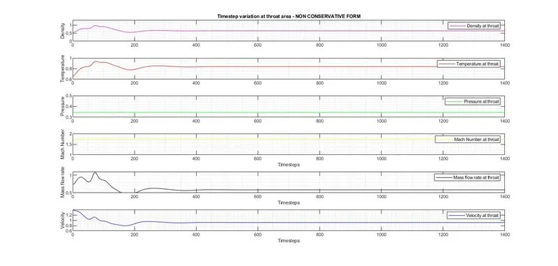
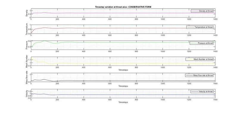
Time steps variation of primitive variables at Throat area
Non Conservative form
Conservative form
Observation:
From the above plots we can conclude that initial variations observed in non nonservative form for a certain period of time makes it consume higher amount of time to acheive stable solution when compared to conservative form.
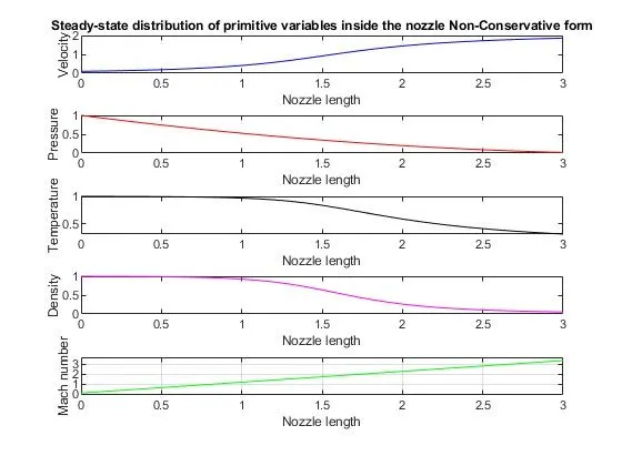
Steady state Variation of primitive variables
Non Conservative form
Conservative Form
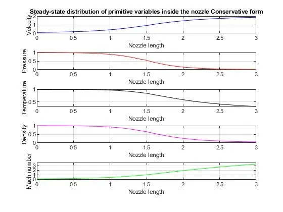
Observation:
Here by observing the above plots we could see that both the forms are in same phase giving the exact same solution for all the values.
Mass flow rates at different Timesteps:
Non Conservative form:
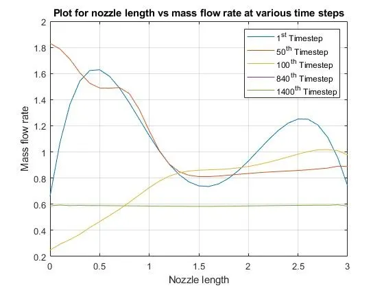
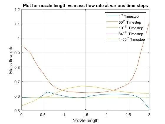
Observation:
Above plots shows that Mass Flow Rate at different Time steps along the Distance oscillates initially, however the solution becomes stable after the 840th Timestep for both the forms attaining a constant value at 1400th time step.
COMPARISON PLOT of Normalized Mass Flow Rate of both NON CONSERVATIVE & CONSERVATIVE FORMS:
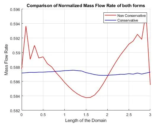
Observation:
Eventhough the final solution of both the forms are almost similar, the Non Conservative form oscillates much when compared to Conservative form. The latter also gives almost stable solution along the length. By this we can conclude that Conservative form attains stability in lesser number of iterations with earliest time.
Grid Dependence test
Observation:
Grid dependency is an important factor to determine whether the problem can be solved faster. So here we increased the Grid points from 31 to 61.
It is clear from the above table that the values are almost same along all the Primitive Variables for both the forms even when the Grid points(n) is changed from 31 to 61 showcasing that it doesn't get affected by the increase of Grid points.
So we can safely conclude that the above problem is Grid Dependant.
CONCLUSION:
Cumulating all the above results we can evidently conclude that Conservative form converges slightly faster than Non Conservative form offering stable solution along the simulation. Yet both the forms are dependable in calculating the solutions which is almost precise.