Week 5 - Rayleigh Taylor Instability

The Rayleigh–Taylor instability, or RT instability (after Lord Rayleigh and G. I. Taylor), is an instability of an interface between two fluids of different densities which occurs when the lighter fluid is pushing the heavier fluid. Examples include the behavior of water suspended above oil in the gravity of Earth,mushroom clouds like those from volcanic eruptions and atmospheric nuclear explosions, supernova explosions in which expanding core gas is accelerated into denser shell gas, instabilities in plasma fusion reactors and inertial confinement fusion.

Water suspended atop oil is an everyday example of Rayleigh–Taylor instability, and it may be modeled by two completely plane-parallel layers of immiscible fluid, the denser fluid on top of the less dense one and both subject to the Earth's gravity. The equilibrium here is unstable to any perturbations or disturbances of the interface: if a parcel of heavier fluid is displaced downward with an equal volume of lighter fluid displaced upwards, the potential energy of the configuration is lower than the initial state. Thus the disturbance will grow and lead to a further release of potential energy, as the denser material moves down under the (effective) gravitational field, and the less dense material is further displaced upwards. This was the set-up as studied by Lord Rayleigh.The important insight by G. I. Taylor was his realisation that this situation is equivalent to the situation when the fluids are accelerated, with the less dense fluid accelerating into the denser fluid. This occurs deep underwater on the surface of an expanding bubble and in a nuclear explosion.

As the RT instability develops, the initial perturbations progress from a linear growth phase into a non-linear growth phase, eventually developing "plumes" flowing upwards (in the gravitational buoyancy sense) and "spikes" falling downwards. In the linear phase, the fluid movement can be closely approximated by linear equations, and the amplitude of perturbations is growing exponentially with time. In the non-linear phase, perturbation amplitude is too large for a linear approximation, and non-linear equations are required to describe fluid motions. In general, the density disparity between the fluids determines the structure of the subsequent non-linear RT instability flows (assuming other variables such as surface tension and viscosity are negligible here). The difference in the fluid densities divided by their sum is defined as the Atwood number, A. For A close to 0, RT instability flows take the form of symmetric "fingers" of fluid; for A close to 1, the much lighter fluid "below" the heavier fluid takes the form of larger bubble-like plumes.

This process is evident not only in many terrestrial examples, from salt domes to weather inversions, but also in astrophysics and electrohydrodynamics. For example, RT instability structure is evident in the Crab Nebula, in which the expanding pulsar wind nebula powered by the Crab pulsar is sweeping up ejected material from the supernova explosion 1000 years ago. The RT instability has also recently been discovered in the Sun's outer atmosphere, or solar corona, when a relatively dense solar prominence overlies a less dense plasma bubble. This latter case resembles magnetically modulated RT instabilities.

Note that the RT instability is not to be confused with the Plateau–Rayleigh instability (also known as Rayleigh instability) of a liquid jet. This instability, sometimes called the hosepipe (or firehose) instability, occurs due to surface tension, which acts to break a cylindrical jet into a stream of droplets having the same total volume but higher surface area.

Many people have witnessed the RT instability by looking at a lava lamp, although some might claim this is more accurately described as an example of Rayleigh–Bénard convection due to the active heating of the fluid layer at the bottom of the lamp.

Stages of development and eventual evolution into turbulent mixing

The evolution of the RTI follows four main stages. In the first stage, the perturbation amplitudes are small when compared to their wavelengths, the equations of motion can be linearized, resulting in exponential instability growth. In the early portion of this stage, a sinusoidal initial perturbation retains its sinusoidal shape. However, after the end of this first stage, when non-linear effects begin to appear, one observes the beginnings of the formation of the ubiquitous mushroom-shaped spikes (fluid structures of heavy fluid growing into light fluid) and bubbles (fluid structures of light fluid growing into heavy fluid). The growth of the mushroom structures continues in the second stage and can be modeled using buoyancy drag models, resulting in a growth rate that is approximately constant in time. At this point, nonlinear terms in the equations of motion can no longer be ignored. The spikes and bubbles then begin to interact with one another in the third stage. Bubble merging takes place, where the nonlinear interaction of mode coupling acts to combine smaller spikes and bubbles to produce larger ones. Also, bubble competition takes places, where spikes and bubbles of smaller wavelength that have become saturated are enveloped by larger ones that have not yet saturated. This eventually develops into a region of turbulent mixing, which is the fourth and final stage in the evolution. It is generally assumed that the mixing region that finally develops is self-similar and turbulent, provided that the Reynolds number is sufficiently large.

Linear stability analysis

The inviscid two-dimensional Rayleigh–Taylor (RT) instability provides an excellent springboard into the mathematical study of stability because of the simple nature of the base state. This is the equilibrium state that exists before any perturbation is added to the system, and is described by the mean velocity field where the gravitational field is An interface at separates the fluids of densities in the upper region, and in the lower region. In this section it is shown that when the heavy fluid sits on top, the growth of a small perturbation at the interface is exponential, and takes place at the rate

where is the temporal growth rate, {\displaystyle \alpha \,} is the spatial wavenumber and is the Atwood number.

The time evolution of the free interface elevation initially at is given by:

which grows exponentially in time. Here B is the amplitude of the initial perturbation, and denotes the real part of the complex valued expression between brackets.

In general, the condition for linear instability is that the imaginary part of the "wave speed" c is positive. Finally, restoring the surface tension makes c² less negative and is therefore stabilizing. Indeed, there is a range of short waves for which the surface tension stabilizes the system and prevents the instability forming.

When the two layers of the fluid are allowed to have a relative velocity, the instability is generalized to the Kelvin–Helmholtz–Rayleigh–Taylor instability, which includes both the Kelvin–Helmholtz instability and the Rayleigh–Taylor instability as special cases. It was recently discovered that the fluid equations governing the linear dynamics of the system admit a parity-time symmetry, and the Kelvin–Helmholtz–Rayleigh–Taylor instability occurs when and only when the parity-time symmetry breaks spontaneously.

Vorticity explanation

The RT instability can be seen as the result of baroclinic torque created by the misalignment of the pressure and density gradients at the perturbed interface, as described by the two-dimensional inviscid vorticity equation, , where ω is vorticity, ρ density and p is the pressure. In this case the dominant pressure gradient is hydrostatic, resulting from the acceleration.

When in the unstable configuration, for a particular harmonic component of the initial perturbation, the torque on the interface creates vorticity that will tend to increase the misalignment of the gradient vectors. This in turn creates additional vorticity, leading to further misalignment. This concept is depicted in the figure, where it is observed that the two counter-rotating vortices have velocity fields that sum at the peak and trough of the perturbed interface. In the stable configuration, the vorticity, and thus the induced velocity field, will be in a direction that decreases the misalignment and therefore stabilizes the system.

Late-time behaviour

The analysis in the previous section breaks down when the amplitude of the perturbation is large. The growth then becomes non-linear as the spikes and bubbles of the instability tangle and roll up into vortices. Then, as in the figure, numerical simulation of the full problem is required to describe the system.

Spaceclaim geometry

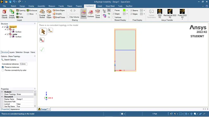
Defining the baseline mesh of 0.5mm

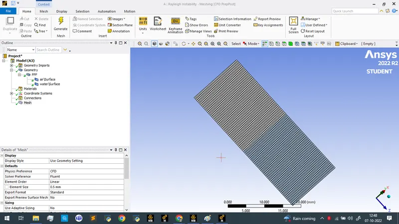
Mesh metrics for baseline mesh

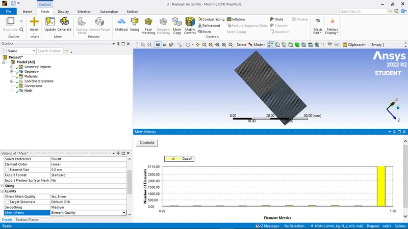
Specifying the general conditions in Fluent

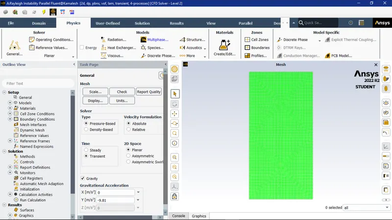
Solver - Pressure based , transient solver with Absolute velocity formulation with Gravity of value 9.81 enabled

Viscous model - Laminar

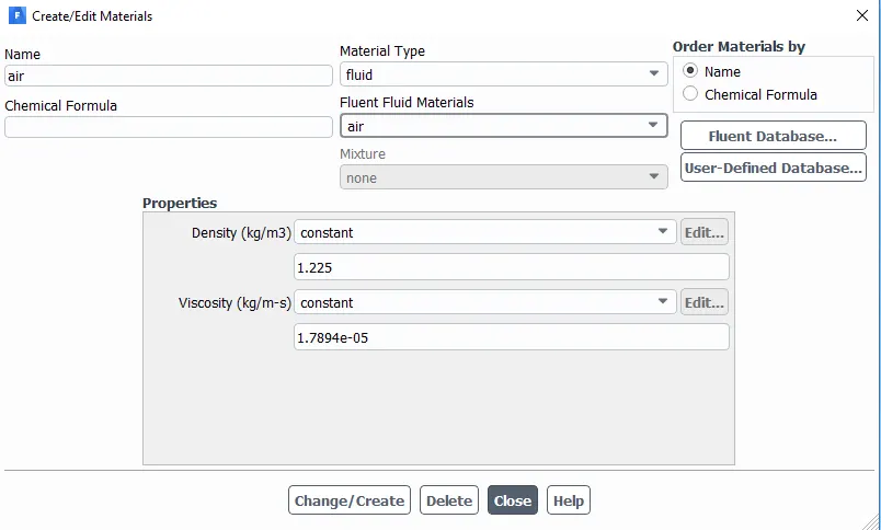
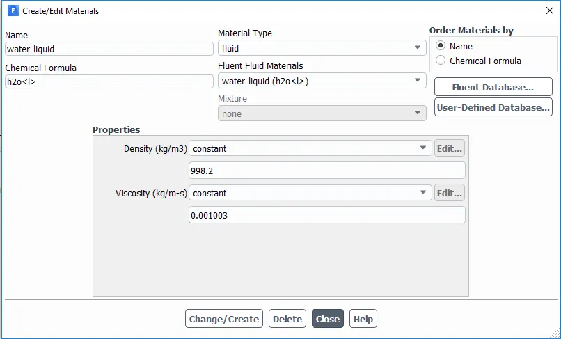
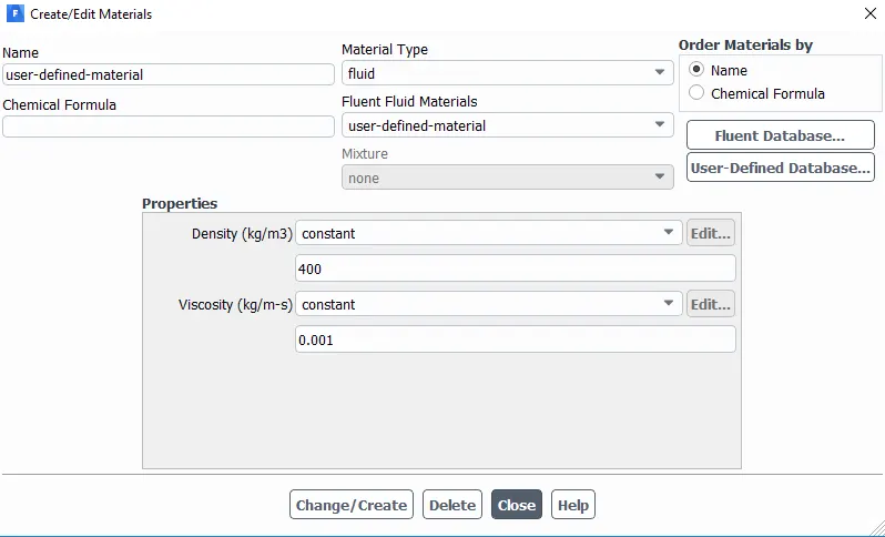
Material properties of air, water and user-defined material:

Multiphase models

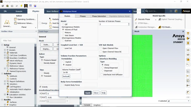
Primary and secondary phases air and water

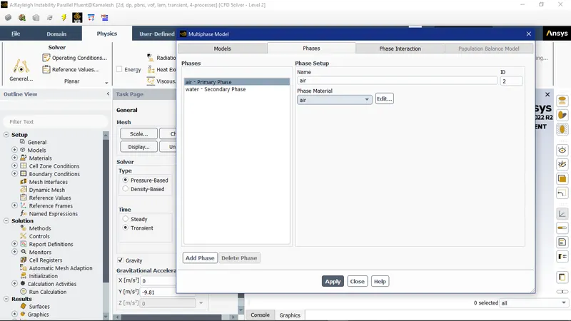
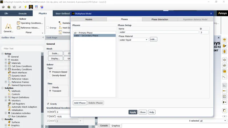
Phases of volume fraction

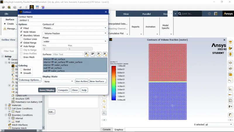
After initializing the solution the surfaces are patched.

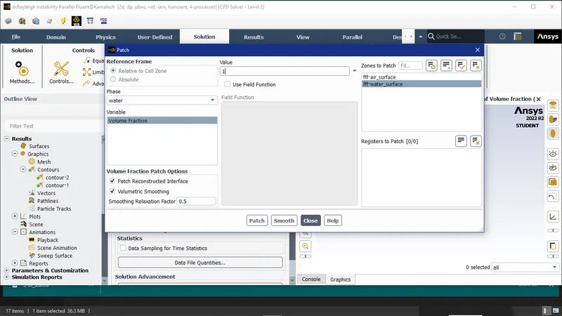
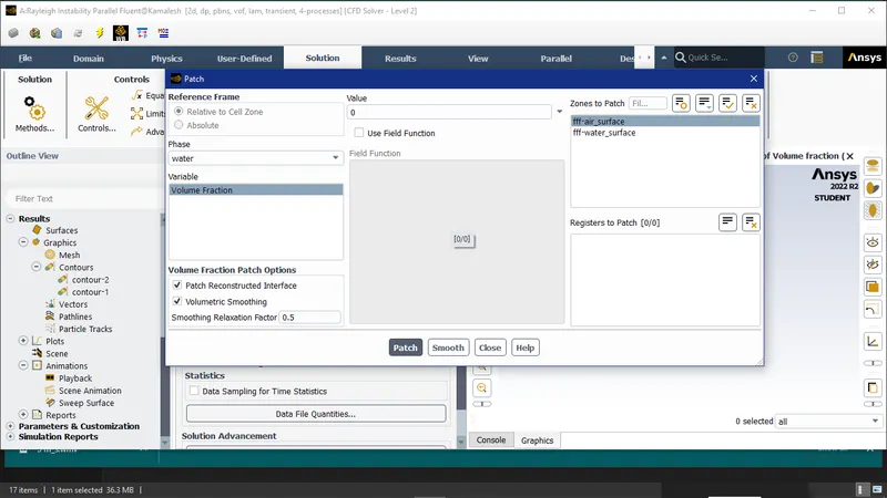
Upon patching the contour surface is created and displayed

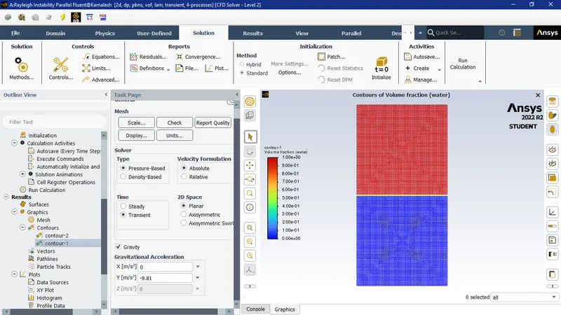
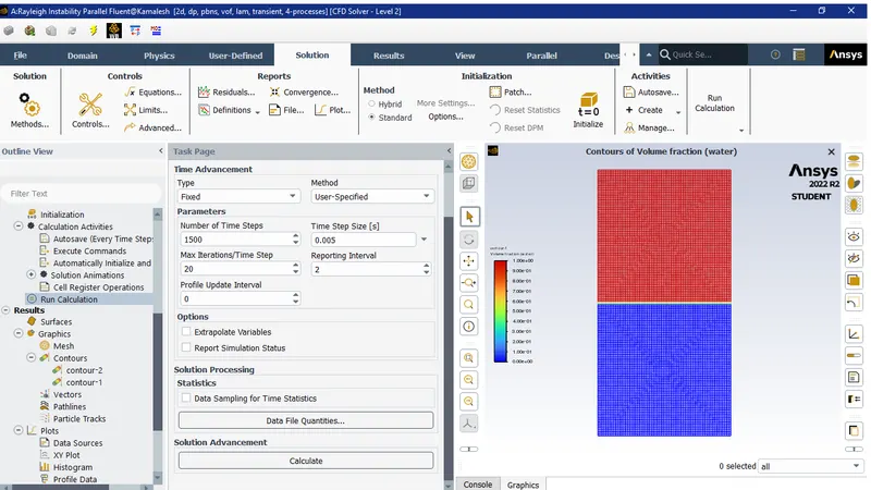
Also an animation is defined to witness the Rayleigh Taylor Instability after which the calculation time steps are defined to calculate the solution

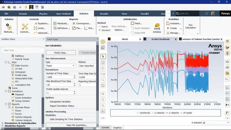
Scaled residuals

Simulation video link for baseline mesh: https://youtu.be/ljhyHgoxxlw

Mesh Refinement

Case 1

The baseline mesh is refined with mesh size 0,3 mm and the solution is calculated for the above conditions and the simulation is recorded as an animation.

Simulation video link for refined mesh: https://youtu.be/uLMH85Wb1LM

Case 2:

The baseline mesh is refined and the solution is calculated for the above conditions with density = 400 kg/m³, viscosity = 0.001 kg/m-s and the simulation is recorded as an animation.

Scaled Residuals

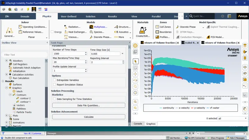
Simulation video link for refined mesh with user defined material: https://youtu.be/cjg2dp6CUOI

Observation:

Finer mesh captures the instability better than the coarse mesh , but it takes more time for the heavier fluid to settle down. So it is computationally expensive but produces results with better accuracy.

Since the simulation involves capturing instabilities which are changing in an unpredictable manner as a function of time , transient approach is preferred over steady state approach.

Atwood Number

It is a dimensionless number that is used to study hydrodynamic instabilities in density stratified flows.

`A=(ρ_1-ρ_2)/(ρ_1+ρ_2)`

where,

`ρ_1`is density of the heavier fluid

`ρ_2`is density of the lighter fluid

For Air-water RT instability,

`rho_1`= 998.2 `(kg)/(m^3)` [density of water]

`rho_2`= 1.225 `(kg)/(m^3)` [density of air]

A = (998.2-1.225)/(998.2+1.225)

A = 0.998

For water- UD material RT instability,

`rho_1` = 998.2 `(kg)/(m^3)` [density of water]

`rho_2 = 400 (kg)/(m^3)` [density of user defined material]

A = (998.2-400)/(998.2+400)

A = 0.428

Behaviour of RT Instability on variation of Atwood number:

RTI evolves in three distinct stages: Linear stability , mushroom head(falling) or bubble(rising) formation , long term evolution due to bubble merging and mixing. For low Atwood number, bubble and mushroom head shape is relatively symmetrical, the disturbances or perturbations are linear for a larger time. In contrast, for large Atwood number, bubble and mushroom head shape is less symmetrical, also it occurs very rapidly at an accelerating rate which leads to a non linear growth rate.

Conclusion:

Atwood number forms a basis to compare and study research papers based on RT Instabilty. Thus we can use these papers to validate our results for beetter accuracy.