Project 2 - Rankine cycle Simulator
RANKINE CYCLE
The Rankine cycle is an idealized thermodynamic cycle describing the process by which certain heat engines, such as steam turbines or reciprocating steam engines, allow mechanical work to be extracted from a fluid as it moves between a heat source and heat sink. The Rankine cycle is named after William John Macquorn Rankine, a Scottish polymath professor at Glasgow University.
Heat energy is supplied to the system via a boiler where the working fluid (typically water) is converted to a high pressure gaseous state (steam) in order to turn a turbine. After passing over the turbine the fluid is allowed to condense back into a liquid state as waste heat energy is rejected before being returned to boiler, completing the cycle. Friction losses throughout the system are often neglected for the purpose of simplifying calculations as such losses are usually much less significant than thermodynamic losses, especially in larger systems.
Description
The Rankine cycle closely describes the process by which steam engines commonly found in thermal power generation plants harness the thermal energy of a fuel or other heat source to generate electricity. Possible heat sources include combustion of fossil fuels such as coal, natural gas, or oil, renewable fuels like biomass or ethanol, nuclear fission, and concentrated solar power. Common heat sinks include ambient air above or around a facility and bodies of water such as rivers, ponds, and oceans.
The ability of a Rankine engine to harness energy depends on the relative temperature difference between the heat source and heat sink. The greater the differential, the more mechanical power can be efficiently extracted out of heat energy, as per Carnot's theorem.
The efficiency of the Rankine cycle is limited by the high heat of vaporization of the working fluid. Unless the pressure and temperature reach super critical levels in the boiler, the temperature range that the cycle can operate over is quite small: Steam turbine entry temperatures are typically around 565 °C and condenser temperatures are around 30 °C.This gives a theoretical maximum Carnot efficiency for the turbine alone of about 63.8% compared with an actual overall thermal efficiency of less than 50% for typical power stations. This low steam turbine entry temperature (compared to a gas turbine) is why the Rankine (steam) cycle is often used as a bottoming cycle to recover otherwise rejected heat in combined-cycle gas turbine power stations.
Rankine engines generally operate in a closed loop where the working fluid is reused. The water vapor with condensed droplets often seen billowing from power stations is created by the cooling systems (not directly from the closed-loop Rankine power cycle). This 'exhaust' heat is represented by the "Qout" flowing out of the lower side of the cycle shown in the T–s diagram below. Cooling towers operate as large heat exchangers by absorbing the latent heat of vaporization of the working fluid and simultaneously evaporating cooling water to the atmosphere.
While many substances can be used as the working fluid, water is usually chosen for its simple chemistry, relative abundance, low cost, and thermodynamic properties. By condensing the working steam vapor to a liquid the pressure at the turbine outlet is lowered and the energy required by the feed pump consumes only 1% to 3% of the turbine output power and these factors contribute to a higher efficiency for the cycle. The benefit of this is offset by the low temperatures of steam admitted to the turbine(s). Gas turbines, for instance, have turbine entry temperatures approaching 1500 °C. However, the thermal efficiency of actual large steam power stations and large modern gas turbine stations are similar.
The four processes in the Rankine cycle
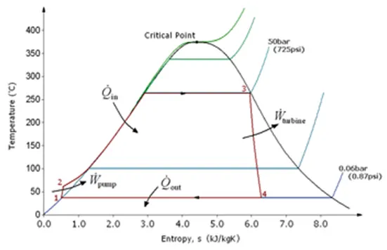
T–s diagram of a typical Rankine cycle operating between pressures of 0.06 bar and 50 bar. Left from the bell-shaped curve is liquid, right from it is gas, and under it is saturated liquid–vapour equilibrium.
There are four processes in the Rankine cycle. The states are identified by numbers (in brown) in the T–s diagram.
- Process 1–2: The working fluid is pumped from low to high pressure. As the fluid is a liquid at this stage, the pump requires little input energy. Process 1-2 is isentropic compression.
- Process 2–3: The high-pressure liquid enters a boiler, where it is heated at constant pressure by an external heat source to become a dry saturated vapour. The input energy required can be easily calculated graphically, using an enthalpy–entropy chart (h–s chart, or Mollier diagram), or numerically, using steam tables or software. Process 2-3 is constant pressure heat addition in boiler.
- Process 3–4: The dry saturated vapour expands through a turbine, generating power. This decreases the temperature and pressure of the vapour, and some condensation may occur. The output in this process can be easily calculated using the chart or tables noted above. Process 3-4 is isentropic expansion.
- Process 4–1: The wet vapour then enters a condenser, where it is condensed at a constant pressure to become a saturated liquid. Process 4-1 is constant pressure heat rejection in condenser.
In an ideal Rankine cycle the pump and turbine would be isentropic, i.e., the pump and turbine would generate no entropy and hence maximize the net work output. Processes 1–2 and 3–4 would be represented by vertical lines on the T–s diagram and more closely resemble that of the Carnot cycle. The Rankine cycle shown here prevents the state of the working fluid from ending up in the superheated vapor region after the expansion in the turbine,which reduces the energy removed by the condensers.
The actual vapor power cycle differs from the ideal Rankine cycle because of irreversibilities in the inherent components caused by fluid friction and heat loss to the surroundings; fluid friction causes pressure drops in the boiler, the condenser, and the piping between the components, and as a result the steam leaves the boiler at a lower pressure; heat loss reduces the net work output, thus heat addition to the steam in the boiler is required to maintain the same level of net work output.
Variables
|
`dot Q` |
Heat flow rate to or from the system (energy per unit time) |
|
`dot m` |
Mass flow rate (mass per unit time) |
|
`dot W` |
Mechanical power consumed by or provided to the system (energy per unit time) |
|
`eta_(therm)` |
Ƞtherm Thermodynamic efficiency of the process (net power output per heat input, dimensionless) |
|
`eta_(pump),eta_(turb)` |
Ƞpump , Ƞturb Isentropic efficiency of the compression (feed pump) and expansion (turbine) processes, dimensionless |
|
`h_1,h_2,h_3,h_4` |
h1,h2,h3,h4 The "specific enthalpies" at indicated points on the T–s diagram |
|
`h_(4s)` |
h4sThe final "specific enthalpy" of the fluid if the turbine were isentropic |
|
`p_1,p_2` |
p1,p2The pressures before and after the compression process |
Equations
In general, the efficiency of a simple Rankine cycle can be written as
`eta _{\text{therm}}={\frac {{\dot {W}}_{\text{thermal}}-{\dot {W}}}{{\dot {Q}}_{\text{in}}}}\approx {\frac {{\dot {W}}_{\text{turb}}}{{\dot {Q}}_{\text{in}}}}.}`
Each of the next four equation is derived from the energy and mass balance for a control volume. `eta_(therm)` defines the thermodynamic efficiency of the cycle as the ratio of net power output to heat input. As the work required by the pump is often around 1% of the turbine work output, it can be simplified.
`dot Q_(In)/dot m =h_3-h_2`
`dot Q_(out)/dotm = h_4-h_1`
`dot W_(pump)/dot m = h_2-h_1`
`dot W_(turb)/dot m = h_3-h_4`
When dealing with the efficiencies of the turbines and pumps, an adjustment to the work terms must be made:
`{ {\frac {{\dot {W}}_{\text{pump}}}{\dot {m}}}=h_{2}-h_{1}\approx {\frac {v_{1}\Delta p}{\eta _{\text{pump}}}}={\frac {v_{1}(p_{2}-p_{1})}{\eta _{\text{pump}}}}}`

Real Rankine cycle (non-ideal)
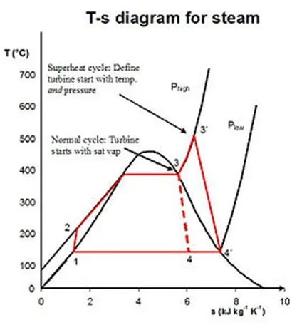
Rankine cycle with superheat
In a real power-plant cycle (the name "Rankine" cycle is used only for the ideal cycle), the compression by the pump and the expansion in the turbine are not isentropic. In other words, these processes are non-reversible, and entropy is increased during the two processes. This somewhat increases the power required by the pump and decreases the power generated by the turbine.
In particular, the efficiency of the steam turbine will be limited by water-droplet formation. As the water condenses, water droplets hit the turbine blades at high speed, causing pitting and erosion, gradually decreasing the life of turbine blades and efficiency of the turbine. The easiest way to overcome this problem is by superheating the steam. On the T-s diagram above, state 3 is at a border of the two-phase region of steam and water, so after expansion the steam will be very wet. By superheating, state 3 will move to the right (and up) in the diagram and hence produce a drier steam after expansion.
Variations of the basic Rankine cycle
The overall thermodynamic efficiency can be increased by increasing the average heat input temperature of that cycle. Increasing the temperature of the steam into the superheat region is a simple way of doing this. There are also variations of the basic Rankine cycle designed to raise the thermal efficiency of the cycle in this way; two of these are described below.
Rankine cycle with reheat
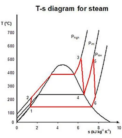
Rankine cycle with reheat
The purpose of a reheating cycle is to remove the moisture carried by the steam at the final stages of the expansion process. In this variation, two turbines work in series. The first accepts vapour from the boiler at high pressure. After the vapor has passed through the first turbine, it re-enters the boiler and is reheated before passing through a second, lower-pressure, turbine. The reheat temperatures are very close or equal to the inlet temperatures, whereas the optimal reheat pressure needed is only one fourth of the original boiler pressure. Among other advantages, this prevents the vapor from condensing during its expansion and thereby reducing the damage in the turbine blades, and improves the efficiency of the cycle, because more of the heat flow into the cycle occurs at higher temperature. The reheat cycle was first introduced in the 1920s, but was not operational for long due to technical difficulties. In the 1940s, it was reintroduced with the increasing manufacture of high-pressure boilers, and eventually double reheating was introduced in the 1950s. The idea behind double reheating is to increase the average temperature. It was observed that more than two stages of reheating are generally unnecessary, since the next stage increases the cycle efficiency only half as much as the preceding stage. Today, double reheating is commonly used in power plants that operate under supercritical pressure.
Regenerative Rankine cycle
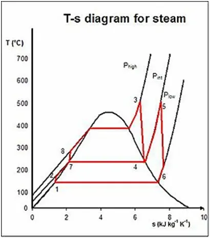
Regenerative Rankine cycle
The regenerative Rankine cycle is so named because after emerging from the condenser (possibly as a sub cooled liquid) the working fluid is heated by steam tapped from the hot portion of the cycle. On the diagram shown, the fluid at 2 is mixed with the fluid at 4 (both at the same pressure) to end up with the saturated liquid at 7. This is called "direct-contact heating". The Regenerative Rankine cycle (with minor variants) is commonly used in real power stations.
Another variation sends bleed steam from between turbine stages to feedwater heaters to preheat the water on its way from the condenser to the boiler. These heaters do not mix the input steam and condensate, function as an ordinary tubular heat exchanger, and are named "closed feedwater heaters".
Regeneration increases the cycle heat input temperature by eliminating the addition of heat from the boiler/fuel source at the relatively low feedwater temperatures that would exist without regenerative feedwater heating. This improves the efficiency of the cycle, as more of the heat flow into the cycle occurs at higher temperature.
Organic Rankine cycle
The organic Rankine cycle (ORC) uses an organic fluid such as n-pentane or toulene in place of water and steam. This allows use of lower-temperature heat sources, such as solar ponds, which typically operate at around 70–90 °C. The efficiency of the cycle is much lower as a result of the lower temperature range, but this can be worthwhile because of the lower cost involved in gathering heat at this lower temperature. Alternatively, fluids can be used that have boiling points above water, and this may have thermodynamic benefits (See, for example, mercuty vapour turbine). The properties of the actuual working fluid have great influence on the quality of steam (vapour) after the expansion step, influencing the design of the whole cycle.
The Rankine cycle does not restrict the working fluid in its definition, so the name "organic cycle" is simply a marketing concept and the cycle should not be regarded as a separate thermodynamic cycle.
Supercritical Rankine cycle
The Rankine cycle applied using a supercritical fluid combines the concepts of heat regeneration and supercritical Rankine cycle into a unified process called the regenerative supercritical cycle (RGSC). It is optimised for temperature sources 125–450 °C.
Rankine Cycle Steam Turbine
This example models a steam turbine system based on the Rankine Cycle. The cycle includes superheating and reheating to prevent condensation at the high-pressure turbine and the low-pressure turbine, respectively. The cycle also has regeneration by passing extracted steam through closed feedwater heaters to warm up the water and improve cycle efficiency.
The Saturated Fluid Chamber block and the Turbine block are custom components based on the Simscape™ Foundation Two-Phase Fluid Library. The Saturated Fluid Chamber block models a separate saturated liquid volume and saturated vapor volume and is used to create the boiler and the condenser.
Feedwater Preheater Subsystem
Steam Boiler Subsystem
Steam Condenser Subsystem
Steam Reheater Subsystem
References
2. rankine-cycle-steam-turbine
Formulae used for calculating various state parameters and other terms in Rankine cycle
%Rankine cycle using matlab

clear all
close all
clc

%The four stages of Rankine cycle are
%1--->2:Isentropic expansion in turbine
%2--->3:Constant pressure heat rejection in condenser
%3--->4:Isentropic pumping process
%4--->1:Constant pressure heat addition

%Printing the stages of Rankine Cycle

fprintf('Rankine Cycle Simulator \n')
fprintf('1--->2:Isentropic expansion in turbine \n')
fprintf('2--->3:Constant pressure heat rejection in condenser \n')
fprintf('3--->4:Isentropic pumping process \n')
fprintf('4--->1:Constant pressure heat addition \n')

%User Input parameters

P1 = input('Enter the pressure at the turbine inlet in bar \n');
T1 = input('Enter the turbine at the turbine inlet in Celsius \n');
P2 = input('Enter the pressure at the turbine outlet or condenser inlet in bar \n');
fprintf('RESULT\n');

% Calculation of Cp value at P1 & P2 for saturated liquid & vapour
CP1_L=XSteam('CpL_p',P1);
CP1_V=XSteam('CpV_p',P1);
CP2_L=XSteam('CpL_p',P2);
CP2_V=XSteam('CpV_p',P2);


%Calculating the parameters at state point 1
fprintf('At State point 1\n');
fprintf('P1 is :%f Bar\n',P1);
fprintf('T1 is :%f degC\n',T1);

H1 = XSteam('h_pt',P1,T1);
S1 = XSteam('s_pt',P1,T1);
Hf1 = XSteam('hL_p',P1);
Hg1 = XSteam('hV_p',P1);
Ts1 = XSteam('Tsat_p',P1);
Sf1 = XSteam('sL_p',P1);
Sg1 = XSteam('sV_p',P1);

fprintf('H1 is :%f kJ/kg\n',H1);
fprintf('S1 is :%f kJ/kg\n\n',S1);

%Calculating the parameters at state point 2
fprintf('At state point 2\n');
fprintf('P2 is : %f Bar\n', P2);

S2 = S1;
fprintf('S2 is : %f kJ/kgK\n', S2);
Sf2 = XSteam('sL_p',P2);
Sg2 = XSteam('sV_p',P2);
if S2 <= Sg2
     x2 = (S2-Sf2)/(Sg2-Sf2);  %Dryness Fraction
else
    x2 =1;
end
fprintf('x2 is :%f \n', x2);
Hf2 = XSteam('hL_p',P2);
Hg2 = XSteam('hV_p',P2);
if(x2<1)
   H2 = Hf2 + x2 * (Hf2-Hg2);
else
   H2=XSteam('h_pT',P2,T2);
end
fprintf('H2 is : %f kJ/kg\n\n', H2)
Ts2 = XSteam('Tsat_p',P2);
%calculating value of T2
if(x2<1)
    T2=Ts2;
else
    %S2=Sg_2+CP2_V*(log(T2/Tsat_P2))
    T2=(Ts2)*exp((S2-Sg_2)/CP2_V);
end
fprintf('T2 is : %f degC \n', T2)

%Calculating the parameters at state point 3
fprintf('At state point 3\n')

H3 = Hf2;
S3 = Sf2;
T3 = Ts2;
fprintf('T3 is : %f degC\n', T3)
P3 = P2;
fprintf('P3 is : %f Bar\n', P3)
V3 = XSteam('vL_p', P3);
Hf3=XSteam('hL_p',P2);
fprintf('H3 is : %f kJ/kg\n', H3)
Sf3=XSteam('sL_p',P2);
fprintf('S3 is : %f kJ/kgK\n\n', S3)


%Calculating the parameters at state point 4
fprintf('At state point 4\n')

P4 = P1;
fprintf('P4 is : %f Bar\n', P4)
S4 = S3;
fprintf('S4 is : %f kJ/kgK\n', S4)
Wp = V3 * (P4 - P3) * 100;
H4 = Wp + H3;
fprintf('H4 is : %f kJ/kg\n', H4)
T4 = XSteam('T_ps',P4,S4);
fprintf('T4 is : %f Deg celsius \n\n', T4)
Hf4=XSteam('hL_p',P1);
Sf4=XSteam('sL_p',P1);

%Temperature space for plotting saturation curves

t = linspace(1, T1, 1000);
for i = 1 : length(t)
     H_L(i) = XSteam('hL_T', t(i));
     H_V(i) = XSteam('hV_T', t(i));
     S_L(i) = XSteam('sL_T', t(i));
     S_V(i) = XSteam('sV_T', t(i));
end

% Plotting T-s Plot

figure(1)
hold on
plot([S1 S2], [T1 T2], 'r', 'linewidth', 2)
text(S1,T1,' 1')
text(S2,T2,' 2')
plot([S2 Sg2], [T2 T2], 'r', 'linewidth', 2)
text(Sg2,Ts2,' 2s')
plot([Sg2 S3], [Ts2 T3], 'r', 'linewidth', 2)
text(S3,T3,' 3')
plot([S3 S4], [T3 T4], 'r', 'linewidth', 2)
text(S4,T4,' 4')
plot([S4 Sf4], [T4 Ts1], 'r', 'linewidth', 2)
text(Sf4,Ts1,' 4s')
plot([Sf4 Sg1], [Ts1 Ts1], 'r', 'linewidth', 2)
text(Sg1,Ts1,' 1s')
plot([Sg1 S1], [Ts1 T1], 'r', 'linewidth', 2)
plot(S_L, t, 'b', 'linestyle','--','linewidth', 1)
plot(S_V, t, 'b', 'linestyle','--','linewidth', 1)

title('T-S Diagram of Ideal Rankine Cycle')
ylabel('Temprature (degC)')
xlabel('Specific Entropy (kJ/kgK)')

% Step 15
% Plotting H-S Plot
figure(2)
hold on
plot([S1 S2], [H1 H2], 'r', 'linewidth', 2)
text(S1,H1,' 1')
text(S2,H2,' 2')
plot([S2 Sg2], [H2 Hg2], 'r', 'linewidth', 2)
text(Sg2,Hg2,' 2s')
plot([Sg2 S3], [Hg2 H3], 'r', 'linewidth', 2)
text(S3,H3,' 3')
plot([S3 S4], [H3 H4], 'r', 'linewidth', 2)
text(S4,H4,' 4')
plot([S4 Sf4], [H4 Hf4], 'r', 'linewidth', 2)
text(Sf4,Hf4,' 4s')
plot([Sf4 Sg1], [Hf4 Hg1], 'r', 'linewidth', 2)
text(Sg1,Hg1,' 1s')
plot([Sg1 S1], [Hg1 H1], 'r', 'linewidth', 2)
plot(S_L, H_L, 'b','linestyle','--', 'linewidth', 1.5)
plot(S_V, H_V, 'b','linestyle','--', 'linewidth', 1.5)
title('H-S Diagram of Ideal Rankine Cycle')
ylabel('Specific Enthalpy (kJ/kg)')
xlabel('Specific Entropy (kJ/kgK)')

% Calculation of Work done, heat, SSC and efficiency
Wt = H1 - H2;
fprintf('Work by turbine is : %f kJ/kg\n', Wt)
fprintf('Work by compressor is : %f kJ/kg\n', Wp)
Wnet = Wt - Wp;
fprintf('Net Work done is : %f kJ/kg\n', Wnet)
Qin = H1 - H4;
eff_thermal = Wnet*100 / Qin ;    % Efficiency
fprintf('Thermal efficiency is : %f', eff_thermal); disp('%')
SSC = 3600 / Wt;    % Specific steam consumption
fprintf('S.S.C is : %f kg/kWh\n\n ', SSC)
%Calculating back work ratio
bw_r = Wp/Wt;
fprintf('bw_r is : %f \n\n', bw_r)
Output Results and Plots
Rankine Cycle Simulator
1--->2:Isentropic expansion in turbine
2--->3:Constant pressure heat rejection in condenser
3--->4:Isentropic pumping process
4--->1:Constant pressure heat addition
Enter the pressure at the turbine inlet in bar
30
Enter the turbine at the turbine inlet in Celsius
400
Enter the pressure at the turbine outlet or condenser inlet in bar
0.05
RESULT
At State point 1
P1 is :30.000000 Bar
T1 is :400.000000 degC
H1 is :3231.571027 kJ/kg
S1 is :6.923259 kJ/kg
At state point 2
P2 is : 0.050000 Bar
S2 is : 6.923259 kJ/kgK
x2 is :0.814256
H2 is : -1835.177974 kJ/kg
T2 is : 32.875490 degC
At state point 3
T3 is : 32.875490 degC
P3 is : 0.050000 Bar
H3 is : 137.765119 kJ/kg
S3 is : 0.476254 kJ/kgK
At state point 4
P4 is : 30.000000 Bar
S4 is : 0.476254 kJ/kgK
H4 is : 140.776056 kJ/kg
T4 is : 32.945189 Deg celsius
Work by turbine is : 5066.749001 kJ/kg
Work by compressor is : 3.010937 kJ/kg
Net Work done is : 5063.738064 kJ/kg
Thermal efficiency is : 163.832869%
S.S.C is : 0.710515 kg/kWh
bw_r is : 0.000594
>>
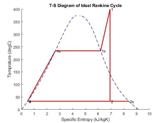
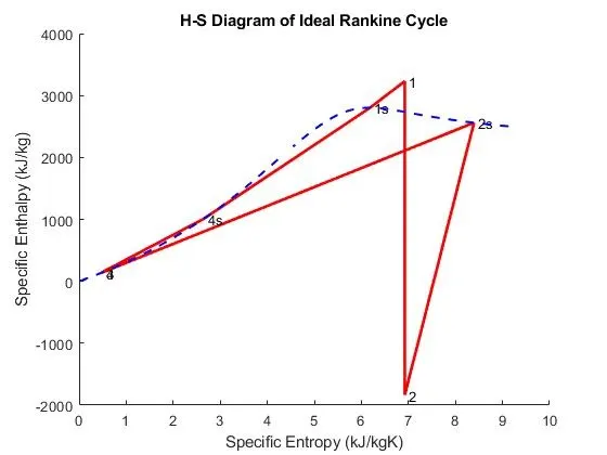
Script Explanation
1. For developing this script,the XSteam.m is required and must be ocated in the same folder as that of the script. The XSteam file is the steam table.
2. Clear the workspace, close all windows and clear all figures and plots.
3. Here the input arguments are defined and taken as user inputs.
4. Cp values at P1 & P2 for saturated liquid & vapour are calculated
5. The state point parameters are calculated and the results are printed.
6. The saturation properties at state points 1,2,3 and 4 are calculated.
7. Similarly the process properties at state points 1,2,3 and 4 are calculated. The pump work is also calculated.
8. Temperature space for plotting saturation curves is defined.
9. The saturation properties of liquid and vapour are calculated for this temperature range. These saturation properties are to be used in plotting the saturation liquid and vapour lines.
10. The T-S and H-S plots for the ideal Rankine cycle are genarated with proper title and labels.
11. Also the values of turbine work,net work,heat input,specific steam consumption and back work ratio are calculated. The results aare then printed.