Week 8 - Simulation of a backward facing step in OpenFOAM

Backward-Facing Step (BFS) flow is one representative model for separation flows, which can be widely seen in aerodynamic flows (airfoil, spoiler, high attack angle process), engine flows, condensers, vehicles (cars, boat), heat transfer systems, and even the flow around buildings, etc. The flow separation after a simple stage will introduce separation bubble formation, evolution and re-attachment process, which is dependent on the BFS geometric design, the inlet and outlet conditions, turbulent intensity, as well as heat transfer conditions. In the past decades, it has been widely studied by various theoretical, experimental and numerical methods.

1. Introduction:

Studying the flow behavior through various structures is an important subject for a CFD engineer. When fluids flow through different geometries, they exhibit different velocity, pressure and flow properties. In this project, Simulation of a flow through backward facing step is done to study the flow of fluids through geometries that have sudden-changing shapes. The simulations are refined using multiple meshes - mesh grading factors inside the BlockMeshDict file of BlockMesh, which is also used to create the geometry to be solved in OpenFOAM.

2. Objective:

1. Analyze and simulate flow through backward facing step.
2. Creating multiple meshes - mesh grading factors : 0.2, 1 and determining how the velocity magnitude profile changes.
3. Measuring the velocity profile at 0.078 m and 0.085 m from the inlet of geometry.
4. Compare velocity magnitude contours near the step region for the above mentioned grading factors.
5. To understand how different quantities like velocity,pressure behaves due to sudden step.

3. Steps to be done:

• Choosing a solver.
• Selecting a solver tutorial to create Geometry and Meshing.
• Setting up Case.
  • Assigning Boundary conditions .
  • Assigning initial conditions.
• Post-processing the results .
• Plotting Results.

4. Choosing a solver:

OpenFOAM software has been used for this project, hence choosing a solver as per our problem is the first essential step towards the study.

Assumptions for the problem :

1. The fluid is Newtonian
2. The flow is incompressible & laminar .
3. Low renolds number.
4. Zero frictional losses

The solver chosen considering above assumptions is icoFoam.

It solves the incompressible laminar Navier-stokes equations (continuity and momentum) using PISO algorithm.

4. a. Selecting Solver tutorial:

The solver tutorial from the incompressible icoFoam called cavity is chosen for the task and its geometry and initial conditions are modified as per the objective.

5. Creating Geometry:

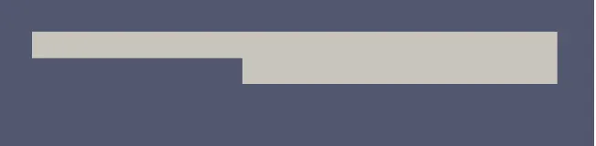
Software file called BlockMeshDict in the tutorials system folder creates the Geometry and mesh, hence this is modified to create the backward facing step. Since blockmeshdict file can create geometries only in block format, we created the blocks and indexed the vertices as shown below.

OpenFoam Block Mesh Geometry

• Mesh Specification:

1. Number of cells along the x direction (longer dimension) = 200.
2. Number of cells along the y direction = 10
3. Use a graded mesh. Grading factor near all walls should be 0.2

we shall perform analysis over different grading factors usch as with a grading factor and simple grading to compare results.

6. Setting up Case:

We now set up the case in blockMeshDict file by assigning Boundary & wall conditions, time step and end time in ControlDict file and initial conditions in the Velocity and pressure file.

6. a. Boundary conditons:

Once the geometry is created, we assign different boundary conditons for the flow to take place within the geometry.

These faces are assigned in the blockMeshDict file as:

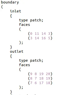
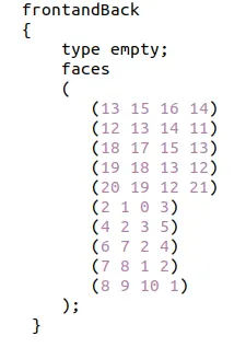
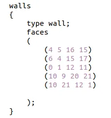
This can be simply represented in the picture below :

6. b. Initial conditions:

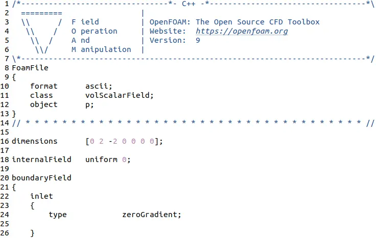
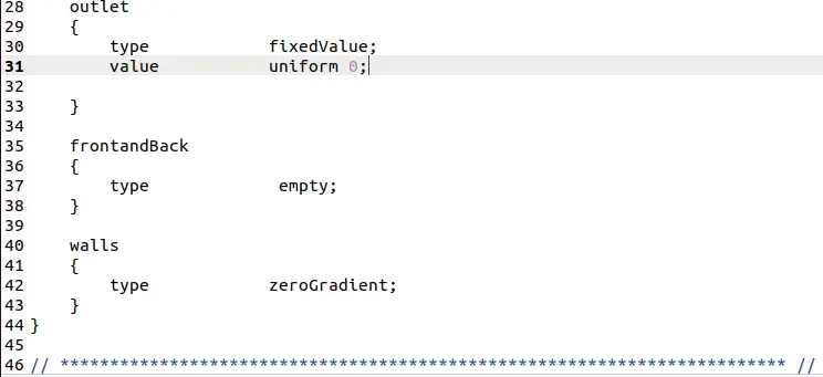
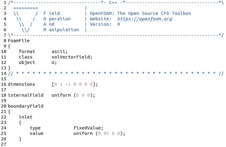
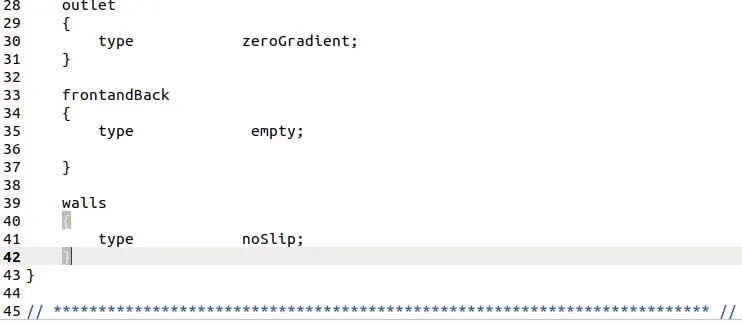
Initial conditions are velocity and pressure, As-per the boundary conditions and the study we wish to perform, the initial conditions are as follows:

Pressure(p)

Velocity(U)

Blockmesh, ControlDict and Transport properties files:

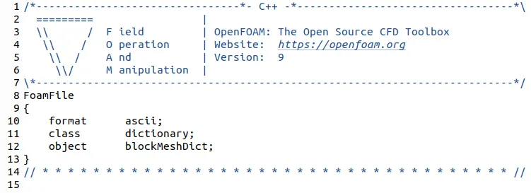
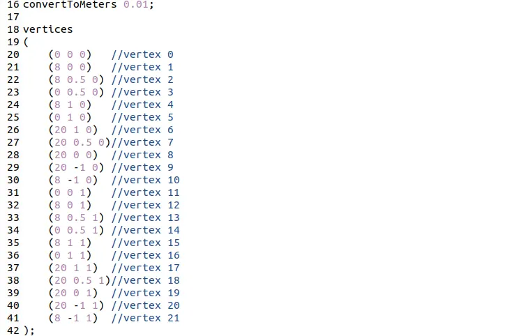
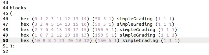
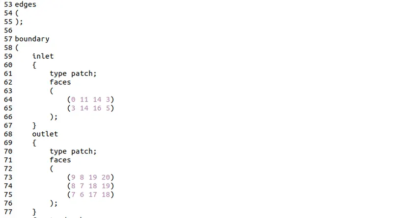
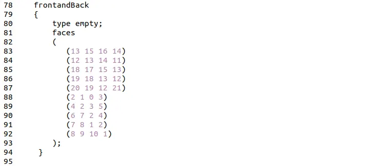
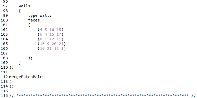
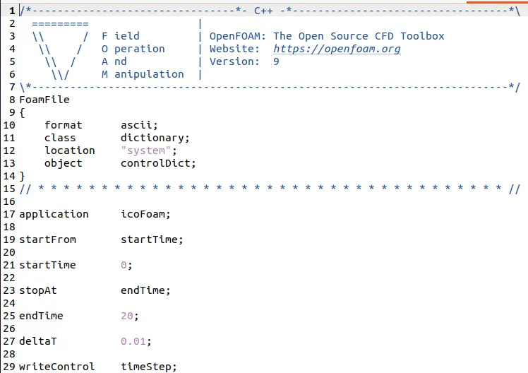
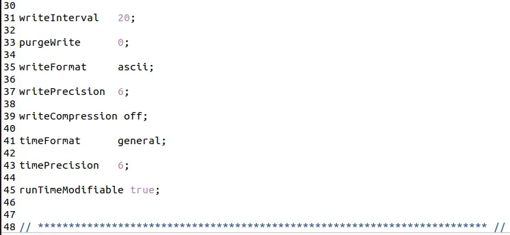
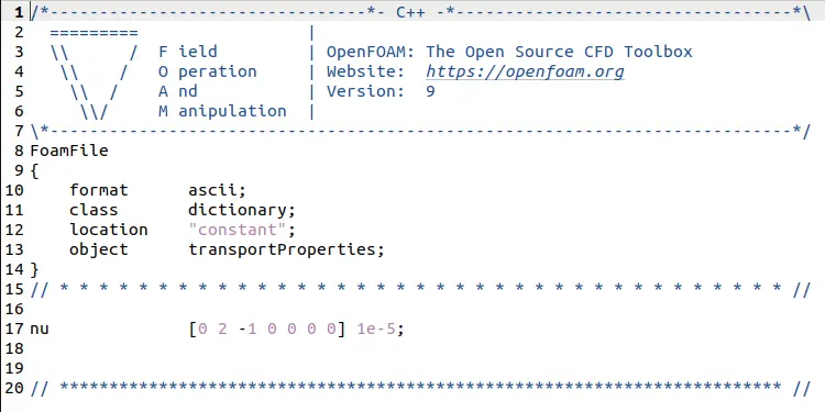
Terminal Screenshots

Creating a copy of cavity

The necessary files are available for the cavity which can be converted into a backward facing step by just changing the values,boundary and initial conditions using the text editor. The terminal should be opened within the run folder.

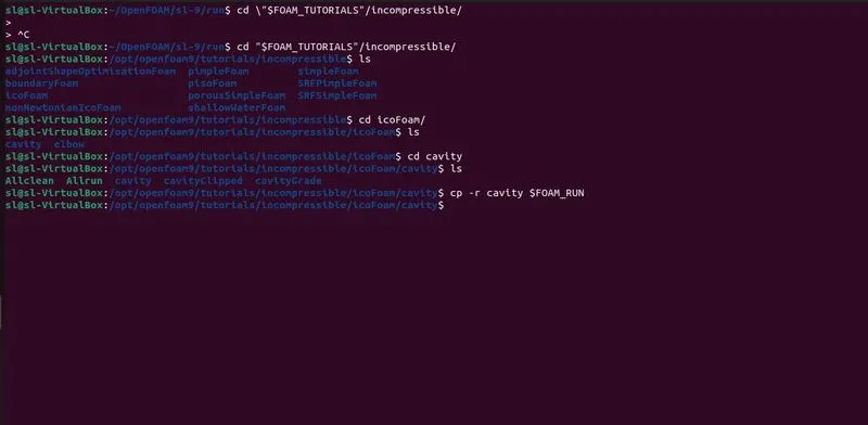
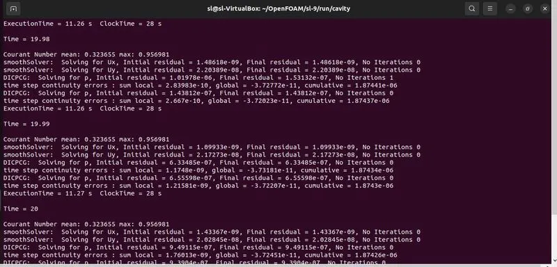
Now a copy of the cavity file will be created within the run folder and the terminal must be opened within the cavity folder. The blockMesh and checkMesh are ran in the terminal after which the icoFoam solver is used in the terminal to calculate the solution.

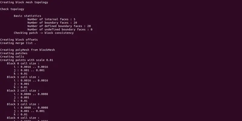
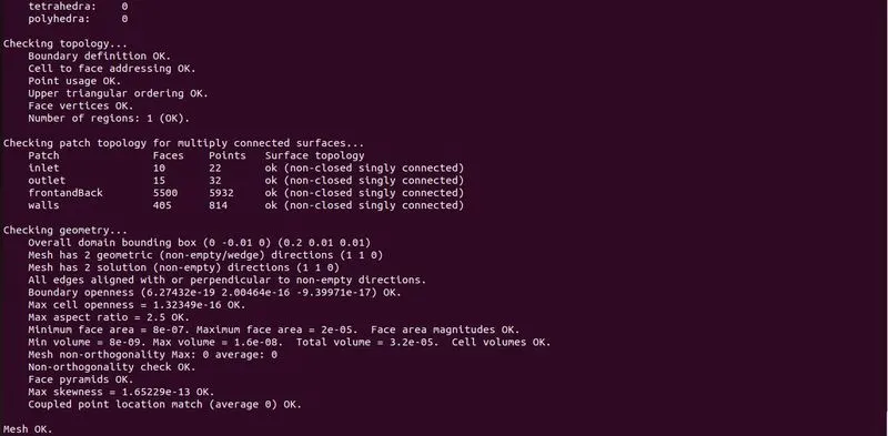
7. Post-Processing Results:

After running the simulations for every grading factor, we post process the results in ParaView software.

a. For grade factor 0.2

Mesh generated

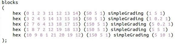
The mesh is created with a grading factor 0.2 and the mesh specifications mentioned in section 5.

The blocks image above are a part of blockmeshdict file and shows the mesh grading and grading factor set on the geometry. we can observe the mesh looks finer and once the mesh is created, we can now run results of simulation in paraview to observe how it looks visually and how the flow seperation takes place in it.

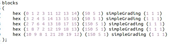
b. For grade factor 1:

Mesh Generated

8. Comparing the plots and final Conclusion:

Comparing the velocity profile near the step region for all the grading factors.

As the fluid flows through a pipe, a boundary layer is created against the walls of the pipe and it builds perpendicular to it, the velocity is slow at the surface and goes on increasing as we move up from the wall.

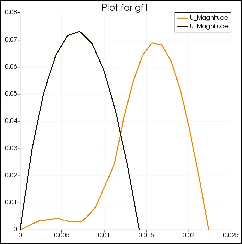
From the contours above, we can see that before the step region the fluid has no obstructon or geometry changes. For x = 0.078 m and 0.085 m with a grading factor 0.2, the velocity behaves like :

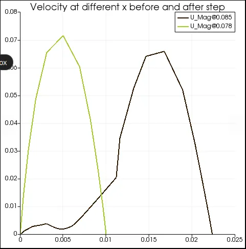
The profile looks close to a parabolic shape with the end points as boundaries and mid-region where the flow speed is maximum.

Once the fluid passes through the step the velocity profile appears.

As the fluid crosses the step region, the area increases. Now looking at the region in graph from 0 to 0.0225, the top part of the geometry after step, comparing to upstream region at x = 0.078 m, The velocity decreases at x= 0.085 m due to increased area. The fluid expands its area of flow and it also mixes with the flow from recirculation zone as it circles up as shown on video above.

For different grading factors, as the mesh becomes more finer at 0.2 we can see the velocity drop curve, its noticeably wider and clearer indication of the result we're anticipating. For grade factor 1 the mesh gets coarser yet its still observable what we concluded from above graph. But as the mesh gets coarser the results are slightly different from finer mesh.

For the region before the step, from 0 to 0.01, this is the recirculation zone, so here the fluid circles back and mixes with the flow and increases with high variation due to crashing on the wall of step and some due to boundary layer and the generation of low pressure zone in that area.

Over all the velocity magnitude profile gives similar results in general but with a mesh grading factor its observed that finer results can be obtained with finer mesh and more accuracy can be aimed in ones solution.

9. Pressure and velocity representations

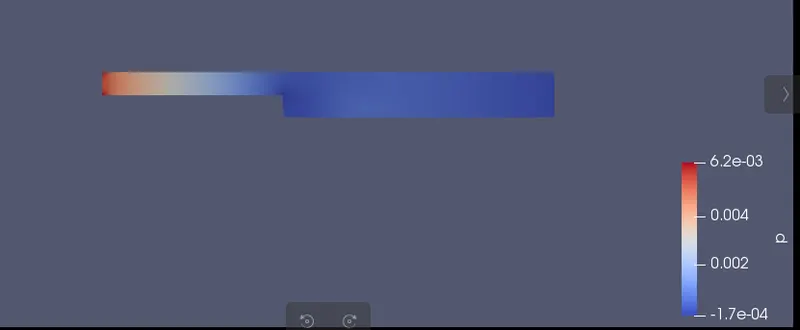
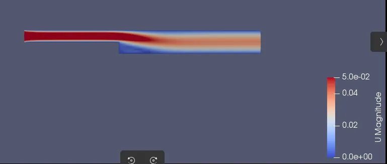
From the simulations, we can see that at the step, the flow gets detached from the wall and is seperated. At the seperation point which we can observe through the different mesh grading factors results, there is slight variation in flow. Now at this seperation point, there is a low pressure region created which causes the flow to recirculate. This gives rise to something called as recirculation zone or wake region.