Week 5.1 - Mid term project - Solving the steady and unsteady 2D heat conduction problem

Conductive Heat transfer

The process by which heat is transferred from the hotter end to the colder end of object is known as conduction.

Heat spontaneously flows from a hotter to a colder body. For example, heat is conducted from the hotplate of an electric stove to the bottom of a saucepan in contact with it. In the absence of an opposing external driving energy source, within a body or between bodies, temperature differences decay over time, and thermal equilibrium is approached, temperature becoming more uniform.

In conduction, the heat flow is within and through the body itself. In contrast, in heat transfer by thermal radiation, the transfer is often between bodies, which may be separated spatially. Heat can also be transferred by a combination of conduction and radiation. In solids, conduction is mediated by the combination of vibrations and collisions of molecules, propagation and collisions of phonons, and diffusion and collisions of free electrons. In gases and liquids, conduction is due to the collisions and diffusion of molecules during their random motion. Photons in this context do not collide with one another, and so heat transport by electromagnetic radiation is conceptually distinct from heat conduction by microscopic diffusion and collisions of material particles and phonons. But the distinction is often not easily observed unless the material is semi-transparent.

In the engineering sciences, heat transfer includes the processes of thermal radiation, convection, and sometimes mass transfer. Usually, more than one of these processes occurs in a given situation.

The conventional symbol for thermal conductivity is k

Overview

On a microscopic scale, conduction occurs within a body considered as being stationary; this means that the kinetic and potential energies of the bulk motion of the body are separately accounted for. Internal energy diffuses as rapidly moving or vibrating atoms and molecules interact with neighbouring particles, transferring some of their microscopic kinetic and potential energies, these quantities being defined relative to the bulk of the body considered as being stationary. Heat is transferred by conduction when adjacent atoms or molecules collide or as several electrons move backwards and forwards from atom to atom in a disorganized way so as not to form a macroscopic electric current, or as photons collide and scatter. Conduction is the most significant means of heat transfer within a solid or between solid objects in thermal contact. Conduction is greater in solids because the network of relatively close fixed spatial relationships between atoms helps to transfer energy between them by vibration.

Thermal contact conductance is the study of heat conduction between solid bodies in contact. A temperature drop is often observed at the interface between the two surfaces in contact. This phenomenon is said to be a result of a thermal contact resistance existing between the contacting surfaces. Interfacial thermal resistance is a measure of an interface's resistance to thermal flow. This thermal resistance differs from contact resistance, as it exists even at atomically perfect interfaces. Understanding the thermal resistance at the interface between two materials is of primary significance in the study of its thermal properties. Interfaces often contribute significantly to the observed properties of the materials.

The inter-molecular transfer of energy could be primarily by elastic impact, as in fluids, or by free-electron diffusion, as in metals, or phonon vibration, as in insulators. In insulators, the heat flux is carried almost entirely by phonon vibrations.

Metals (e.g., copper, platinum, gold, etc.) are usually good conductors of thermal energy. This is due to the way that metals bond chemically: metallic bonds (as opposed to covalent or ionic bonds) have free-moving electrons that transfer thermal energy rapidly through the metal. The electron fluid of a conductive metallic solid conducts most of the heat flux through the solid. Phonon flux is still present but carries less of the energy. Electrons also conduct electric current through conductive solids, and the thermal and electrical conductivities of most metals have about the same ratio. A good electrical conductor, such as copper, also conducts heat well. Thermoelectricity is caused by the interaction of heat flux and electric current. Heat conduction within a solid is directly analogous to diffusion of particles within a fluid, in the situation where there are no fluid currents.

In gases, heat transfer occurs through collisions of gas molecules with one another. In the absence of convection, which relates to a moving fluid or gas phase, thermal conduction through a gas phase is highly dependent on the composition and pressure of this phase, and in particular, the mean free path of gas molecules relative to the size of the gas gap, as given by the Knudsen number {\displaystyle K_{n}}.

To quantify the ease with which a particular medium conducts, engineers employ the thermal conductivity, also known as the conductivity constant or conduction coefficient, k. In thermal conductivity, k is defined as "the quantity of heat, Q, transmitted in time (t) through a thickness (L), in a direction normal to a surface of area (A), due to a temperature difference (ΔT) [...]". Thermal conductivity is a material property that is primarily dependent on the medium's phase, temperature, density, and molecular bonding. Thermal effusivity is a quantity derived from conductivity, which is a measure of its ability to exchange thermal energy with its surroundings.

Steady-state conduction

Steady-state conduction is the form of conduction that happens when the temperature difference(s) driving the conduction are constant, so that (after an equilibration time), the spatial distribution of temperatures (temperature field) in the conducting object does not change any further. Thus, all partial derivatives of temperature concerning space may either be zero or have nonzero values, but all derivatives of temperature at any point concerning time are uniformly zero. In steady-state conduction, the amount of heat entering any region of an object is equal to the amount of heat coming out (if this were not so, the temperature would be rising or falling, as thermal energy was tapped or trapped in a region).

For example, a bar may be cold at one end and hot at the other, but after a state of steady-state conduction is reached, the spatial gradient of temperatures along the bar does not change any further, as time proceeds. Instead, the temperature remains constant at any given cross-section of the rod normal to the direction of heat transfer, and this temperature varies linearly in space in the case where there is no heat generation in the rod.

In steady-state conduction, all the laws of direct current electrical conduction can be applied to "heat currents". In such cases, it is possible to take "thermal resistances" as the analog to electrical resistances. In such cases, temperature plays the role of voltage, and heat transferred per unit time (heat power) is the analog of electric current. Steady-state systems can be modeled by networks of such thermal resistances in series and parallel, in exact analogy to electrical networks of resistors. See purely resistive thermal circuits for an example of such a network.

Transient conduction

During any period in which temperatures changes in time at any place within an object, the mode of thermal energy flow is termed transient conduction. Another term is "non-steady-state" conduction, referring to the time-dependence of temperature fields in an object. Non-steady-state situations appear after an imposed change in temperature at a boundary of an object. They may also occur with temperature changes inside an object, as a result of a new source or sink of heat suddenly introduced within an object, causing temperatures near the source or sink to change in time.

When a new perturbation of temperature of this type happens, temperatures within the system change in time toward a new equilibrium with the new conditions, provided that these do not change. After equilibrium, heat flow into the system once again equals the heat flow out, and temperatures at each point inside the system no longer change. Once this happens, transient conduction is ended, although steady-state conduction may continue if heat flow continues.

If changes in external temperatures or internal heat generation changes are too rapid for the equilibrium of temperatures in space to take place, then the system never reaches a state of unchanging temperature distribution in time and the system remains in a transient state.

An example of a new source of heat "turning on" within an object, causing transient conduction, is an engine starting in an automobile. In this case, the transient thermal conduction phase for the entire machine is over, and the steady-state phase appears, as soon as the engine reaches steady-state operating temperature. In this state of steady-state equilibrium, temperatures vary greatly from the engine cylinders to other parts of the automobile, but at no point in space within the automobile does the temperature increase or decrease. After establishing this state, the transient conduction phase of heat transfer is over.

New external conditions also cause this process: for example, the copper bar in the example steady-state conduction experiences transient conduction as soon as one end is subjected to a different temperature from the other. Over time, the field of temperatures inside the bar reaches a new steady-state, in which a constant temperature gradient along the bar is finally set up, and this gradient then stays constant in space. Typically, such a new steady-state gradient is approached exponentially with time after a new temperature-or-heat source or sinks, has been introduced. When a "transient conduction" phase is over, heat flow may continue at high power, so long as temperatures do not change.

An example of transient conduction that does not end with steady-state conduction, but rather no conduction, occurs when a hot copper ball is dropped into oil at a low temperature. Here, the temperature field within the object begins to change as a function of time, as the heat is removed from the metal, and the interest lies in analyzing this spatial change of temperature within the object over time until all gradients disappear entirely (the ball has reached the same temperature as the oil). Mathematically, this condition is also approached exponentially; in theory, it takes infinite time, but in practice, it is over, for all intents and purposes, in a much shorter period. At the end of this process with no heat sink but the internal parts of the ball (which are finite), there is no steady-state heat conduction to reach. Such a state never occurs in this situation, but rather the end of the process is when there is no heat conduction at all.

The analysis of non-steady-state conduction systems is more complex than that of steady-state systems. If the conducting body has a simple shape, then exact analytical mathematical expressions and solutions may be possible. However, most often, because of complicated shapes with varying thermal conductivities within the shape (i.e., most complex objects, mechanisms or machines in engineering) often the application of approximate theories is required, and/or numerical analysis by computer. One popular graphical method involves the use of Heisler Charts.

Occasionally, transient conduction problems may be considerably simplified if regions of the object being heated or cooled can be identified, for which thermal conductivity is very much greater than that for heat paths leading into the region. In this case, the region with high conductivity can often be treated in the lumped capacitance model, as a "lump" of material with a simple thermal capacitance consisting of its aggregate heat capacity. Such regions warm or cool, but show no significant temperature variation across their extent, during the process (as compared to the rest of the system). This is due to their far higher conductance. During transient conduction, therefore, the temperature across their conductive regions changes uniformly in space, and as a simple exponential in time. An example of such systems is those that follow Newton's law of cooling during transient cooling (or the reverse during heating). The equivalent thermal circuit consists of a simple capacitor in series with a resistor. In such cases, the remainder of the system with a high thermal resistance (comparatively low conductivity) plays the role of the resistor in the circuit.

 The 2d heat transfer steady state equation is specified as

`(del^2T)/(delx^2) + (del^2T)/(dely^2) = 0`

Discretizing the above equation

`(T_L -2T_P+T_R)/(Deltax^2) + (T_T -2T_P+T_B)/(Deltay^2) = 0`

On further simplification

`T_p = 1/K[(T_L+T_R)/(Deltax^2) + (T_T+T_B)/(Deltay^2)]`

where `(Deltax^2Deltay^2)/(2(Deltax^2+Deltay^2)`

The explicit method is used to solve the steady state problem as previous values are known.

Transient heat condition

The 2D transient heat conduction equation is given by

`(delT)/(delt) -alpha((del^2T)/(delx^2) + (del^2T)/(dely^2)) = 0`

Since a time derivative is present a time marching solution is used. To solve the transient problem both implicit and explicit methods are used. The explicit method is used to slove the steady state problem as previous values are known whereas the implicit method is used when only when initial value is known and all the other previous values are unknown.

Discretizing the above equation considering `T_(i,j) = T_p`

`(T_p^(n+1) -T_p^n)/(Deltat) -alpha((del^2T)/(delx^2) + (del^2T)/(dely^2)) = 0`

Using central difference method

`(T_p^(n+1) -T_p^n)/(Deltat) = alpha((T_L -2T_p+T_R)/(Deltax^2) + (T_T -2T_p+T_B)/(Deltay^2))`

This equation is an uncoupled linear equation

Explicit method

`T_p^(n+1) = T_p^n+alphaDeltat((T_L -2T_p+T_R)/(Deltax^2) + (T_T -2T_p+T_B)/(Deltay^2))`

Implicit method

`T_p^(n+1) = T_p^n+alphaDeltat((T_L -2T_p+T_R)/(Deltax^2) + (T_T -2T_p+T_B)/(Deltay^2))^(n+1)`

`K_1 = (alphaDeltat)/(Deltax^2)`

`K_2 = (alphaDeltat)/(Deltay^2)`

CFL = K1+K2

The above three values are the same for both explicit and implicit methods

`T_p^(n+1) = T_p^n+K_1(T_L^(n+1) -2T_p^(n+1)+T_R^(n+1)) +K_2(T_T^(n+1) -2T_p^(n+1)+T_B^(n+1))`

Taking all n+1 terms to one side,expanding and simplyfying we get

`T_p^(n+1)(1+2K_1+2K_2) = T_p^n+K_1(T_L^(n+1) +T_R^(n+1)) +K_2(T_T^(n+1) +T_B^(n+1))`

%Code for steady state approach

clear all
close all
clc

%inputs
x =1:10;
y =1:10;
nx = length(x);
ny = length(y);
dx = abs(x(1)-x(2));
dy = abs(y(1)-y(2));
%BC's
T_t = 600;
T_b = 900;
T_l = 400;
T_r = 800;
T = 300*ones(nx,ny);
T(1,:) = T_t;
T(end,:) = T_b;
T(:,1) = T_l;
T(:,end) = T_r;
T(1,1) = (T_l + T_t)/2;
T(1,nx) = (T_t + T_r)/2;
T(nx,ny) = (T_r + T_b)/2;
T(ny,1) = (T_l + T_b)/2;
T_old = T;
T_initial =T;
k =  (dx^2*dy^2)/(2*(dx^2+dy^2));

error =1;
tol = 1e-4;
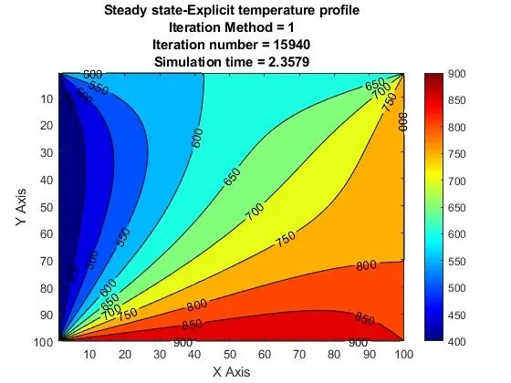
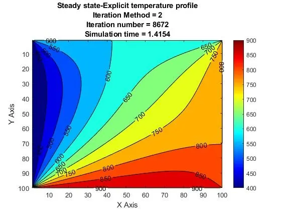
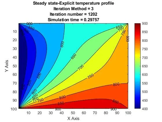
iterative_solver= 2;%Iteration_method = 1-Jacobi ; 2-Gauss seidel ; 3-SOR

%Jacobi method
if iterative_solver == 1
    tic
    it = 1;
    while(error>tol)
     for i = 2:(nx-1)
        for j = 2:(ny-1)
            
            %calculating the temperature of a point using Jacobi method
            term1 = (T_old(i-1,j)+T_old(i+1,j))/(dx^2);
            term2 = (T_old(i,j-1)+T_old(i,j+1))/(dy^2);
            T(i,j) = k*(term1 + term2);
        end
     end
        error = max(max(abs(T_old-T)));
        T_old = T;
        it = it+1;
    end
    time =toc;
    %Gauss Seidel method
  elseif iterative_solver == 2 
    tic
    it = 1;
    while (error > tol)
        for i = 2:(nx-1)
            for j = 2:(ny-1)
                term1 = (T(i-1,j)+T_old(i+1,j))/(dx^2);
                term2 = (T(i,j-1)+T_old(i,j+1))/(dy^2);
                T(i,j) = k*(term1 + term2);
            end
        end
        error = max(max(abs(T-T_old)));
        T_old = T;
        it = it+1;
    end
    time = toc;
    
    %SOR method
  elseif iterative_solver == 3 
      alpha = 1.8;
    tic
    it = 1;
    while (error > tol)
        for i = 2:(nx-1)
            for j = 2:(ny-1)
                term1 = (T(i-1,j)+T_old(i+1,j))/(dx^2);
                term2 = (T(i,j-1)+T_old(i,j+1))/(dy^2);
                T(i,j) = k*(term1 + term2);
                T(i,j) = T_old(i,j)*(1-alpha)+(alpha*T(i,j));
            end
        end
        error = max(max(abs(T-T_old)));
        T_old = T;
        it = it+1;
    end
    time = toc;
end
    
        %Plotting the results
        figure(1)
        [c,h] = contourf(x,y,T);
        clabel(c,h);
        colorbar
        colormap(jet)
        set(gca,'YDIR','reverse');
        xlabel('X Axis');
        ylabel('Y Axis');
        pause(0.03)
        title_text = sprintf('Iteration number = %d',it);
        title({'Steady state-Explicit temperature profile';['Iteration Method = ',num2str(iterative_solver)];title_text;['Simulation time = ',num2str(time)]})
    

%Code for transient conduction using explicit approach
clear all
close all
clc

%inputs
x =1:10;
y =1:10;
nx = length(x);
ny = length(y);
dx = abs(x(1)-x(2));
dy = abs(y(1)-y(2));
alpha = 1.8;
t =1000;
dt=0.1;
nt =1400;

%BC's
T_t = 600;
T_b = 900;
T_l = 400;
T_r = 800;
T = 300*ones(nx,ny);
T(1,:) = T_t;
T(end,:) = T_b;
T(:,1) = T_l;
T(:,end) = T_r;
T(1,1) = (T_l + T_t)/2;
T(1,nx) = (T_t + T_r)/2;
T(nx,ny) = (T_r + T_b)/2;
T(ny,1) = (T_l + T_b)/2;
T_old = T;
T_initial =T;
K1 =  (alpha*dt)/(dx^2);
K2 =  (alpha*dt)/(dy^2);
CFL  = K1+K2;
error =1;
tol = 1e-4;

 it = 1;
for k=1:nt
    
    tic
   
    
     for i = 2:(nx-1)
        for j = 2:(ny-1)
            
            %calculating the temperature of a point using Jacobi method
            term1 = K1*(T_old(i-1,j)-2*T_old(i,j)+T_old(i+1,j));
            term2 = K2*(T_old(i,j-1)-2*T_old(i,j)+T_old(i,j+1));
            T(i,j) = T_old(i,j)+(term1 + term2);
        end
     end
        T_old = T;
        it = it+1;
    
    time =toc;
end

        %Plotting the results
        figure(1)
        [c,h] = contourf(x,y,T);
        clabel(c,h);
        colorbar
        colormap(jet)
        set(gca,'YDIR','reverse');
        xlabel('X Axis');
        ylabel('Y Axis');
        pause(0.03)
        title_text = sprintf('Iteration number = %d',it);
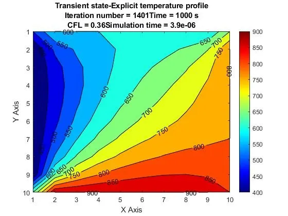
        title({'Transient state-Explicit temperature profile';[title_text,'Time = ',num2str(t),' s'];['CFL = ',num2str(CFL),'Simulation time = ',num2str(time)]})
    

%Code for transient conduction using implicit approach
clear all
close all
clc

%inputs
x =1:10;
y =1:10;
nx = length(x);
ny = length(y);
dx = abs(x(1)-x(2));
dy = abs(y(1)-y(2));
alpha = 1.2;
t = 140;
dt=0.1;
nt =t/dt;

%BC's
T_t = 600;
T_b = 900;
T_l = 400;
T_r = 800;
T = 300*ones(nx,ny);
T(1,:) = T_t;
T(end,:) = T_b;
T(:,1) = T_l;
T(:,end) = T_r;
T(1,1) = (T_l + T_t)/2;
T(1,nx) = (T_t + T_r)/2;
T(nx,ny) = (T_r + T_b)/2;
T(ny,1) = (T_l + T_b)/2;
T_old = T;
T_p_dt =T;
K1 =  (alpha*dt)/(dx^2);
K2 =  (alpha*dt)/(dy^2);
CFL  = K1+K2;

tol = 1e-4;
iterative_solver= 1;%Iteration_method = 1-Jacobi ; 2-Gauss seidel ; 3-SOR

%Jacobi method
if iterative_solver == 1
     tic
    it = 1;
    for k=1:nt
        error =1;
    while(error>tol)
     for i = 2:(nx-1)
        for j = 2:(ny-1)
            
            %calculating the temperature of a point using Jacobi method
            term1 = (1+2*K1+2*K2)^(-1);
            term2 = K1*term1;
            term3= K2*term1;
            h = (T_old(i-1,j)+T_old(i+1,j));
            v = (T_old(i,j-1)+T_old(i,j+1));
            T(i,j) = ((T_p_dt(i,j)*term1) + (h*term2)+(v*term3));
        end
     end
        error = max(max(abs(T_old-T)));
        T_old = T;
        it = it+1;
    end
    
    T_p_dt= T;
    end
    time =toc;
    
%     %Gauss Seidel method
  elseif iterative_solver == 2 
    tic
    it = 1;
      for k=1:nt
        error =1;
        while (error > tol)
        for i = 2:(nx-1)
            for j = 2:(ny-1)
            term1 = (1+2*K1+2*K2)^(-1);
            term2 = K1*term1;
            term3= K2*term1;
            h = (T(i-1,j)+T_old(i+1,j));
            v = (T(i,j-1)+T_old(i,j+1));
            T(i,j) = ((T_p_dt(i,j)*term1) + (h*term2)+(v*term3));
            end
        end
        error = max(max(abs(T-T_old)));
        T_old = T;
        it = it+1;
       end
       T_p_dt= T;
      end
    time = toc;
%     
%     %SOR method
  elseif iterative_solver == 3 
      omega = 1.2;
    tic
    it = 1;
    for k=1:nt
        error =1;
      while (error > tol)
        for i = 2:(nx-1)
            for j = 2:(ny-1)
                term1 = (1+2*K1+2*K2)^(-1);
                term2 = K1*term1;
                term3= K2*term1;
                h = (T(i-1,j)+T_old(i+1,j));
                v = (T(i,j-1)+T_old(i,j+1));
                T(i,j) = ((T_p_dt(i,j)*term1) + (h*term2)+(v*term3));
                T(i,j) = T_old(i,j)*(1-omega)+(omega*T(i,j));
            end
        end
        error = max(max(abs(T-T_old)));
        T_old = T;
        it = it+1;
      end
      T_p_dt= T;
    end
    time = toc;
end
    
        %Plotting the results
        figure(1)
        [c,h] = contourf(x,y,T);
        clabel(c,h);
        colorbar
        colormap(jet)
        set(gca,'YDIR','reverse');
        xlabel('X Axis');
        ylabel('Y Axis');
        pause(0.03)
        title_text = sprintf('Iteration number = %d',it);
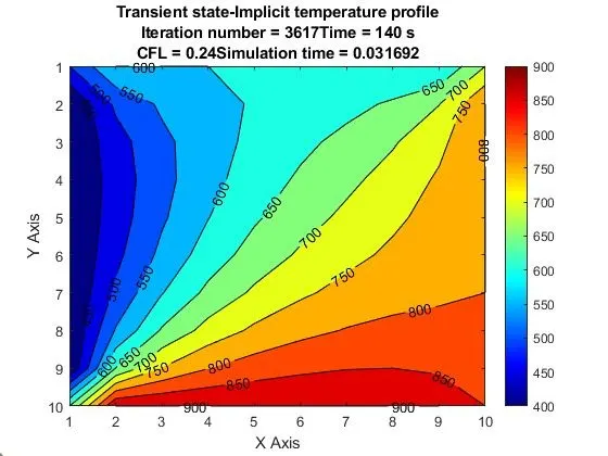
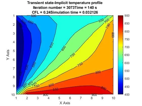
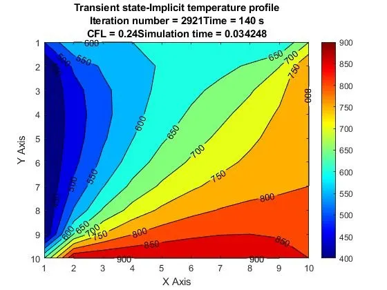
        title({'Transient state-Implicit temperature profile';[title_text,'Time = ',num2str(t),' s'];['CFL = ',num2str(CFL),'Simulation time = ',num2str(time)]})