Week 4 - CHT Analysis on Exhaust port

Importing the exhaust part geometry into spaceclaim

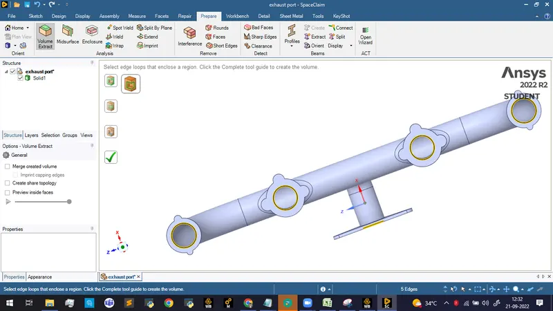
Performing volume extract on the geometry using edge selection option

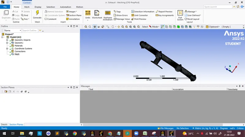
Basic mesh generation

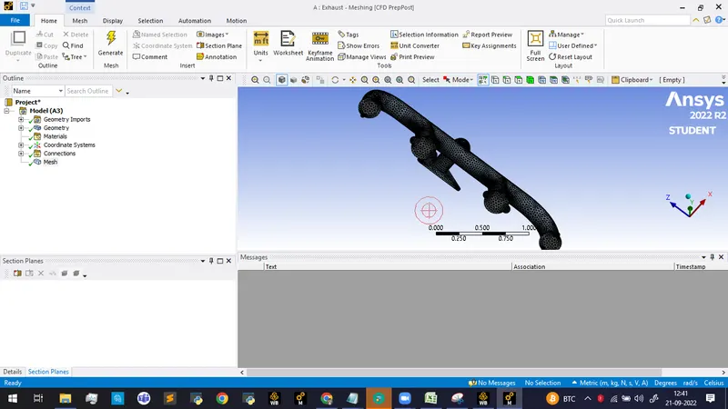
This mesh has no conformance or it is a non conformal mesh. So shared topology has to be performed on the geometry. Enabling shared topology

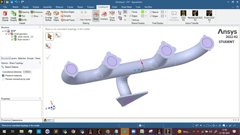
Regenerating the baseline mesh

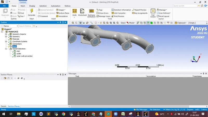
Creating named selections

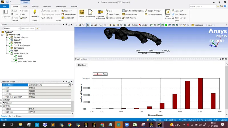
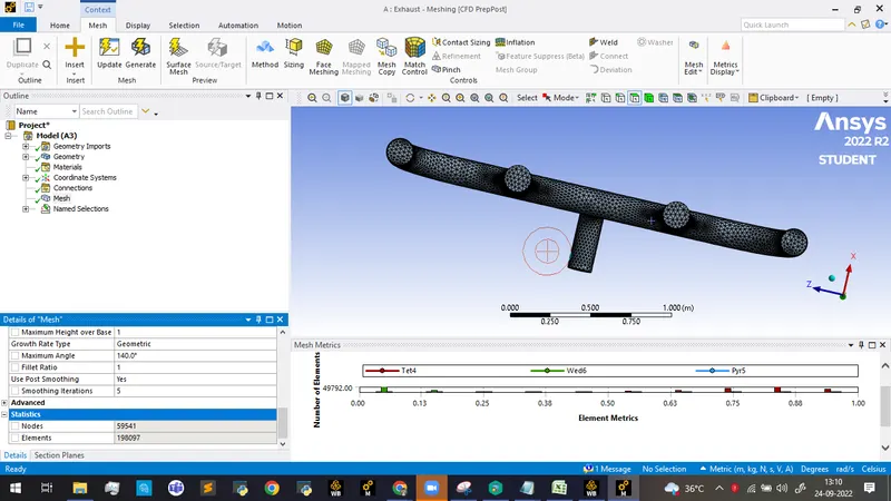
Mesh statistics and metrics for baseline mesh

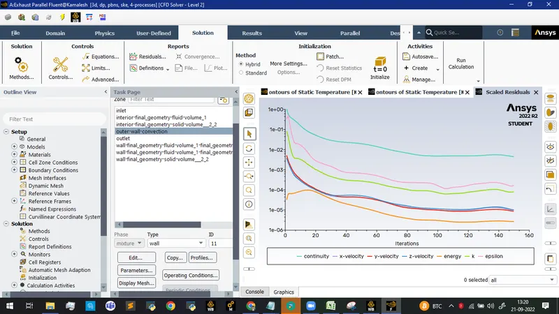
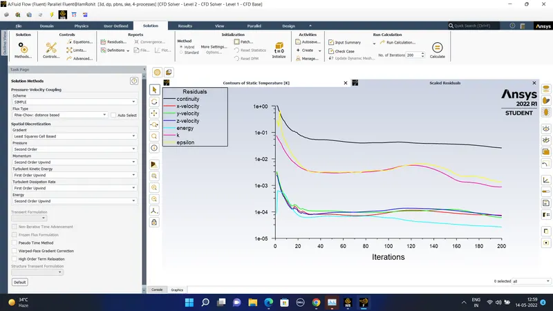
Scaled residuals at velocity 5m/s with pressure based steady state solver,energy equation enabled and k-epslion model.

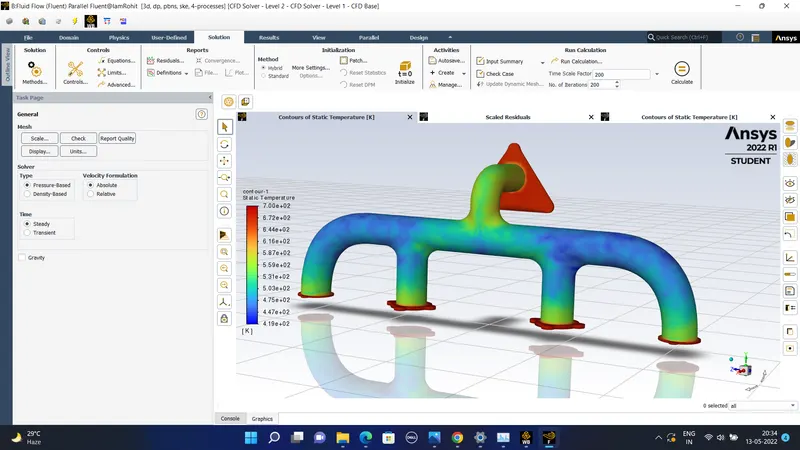
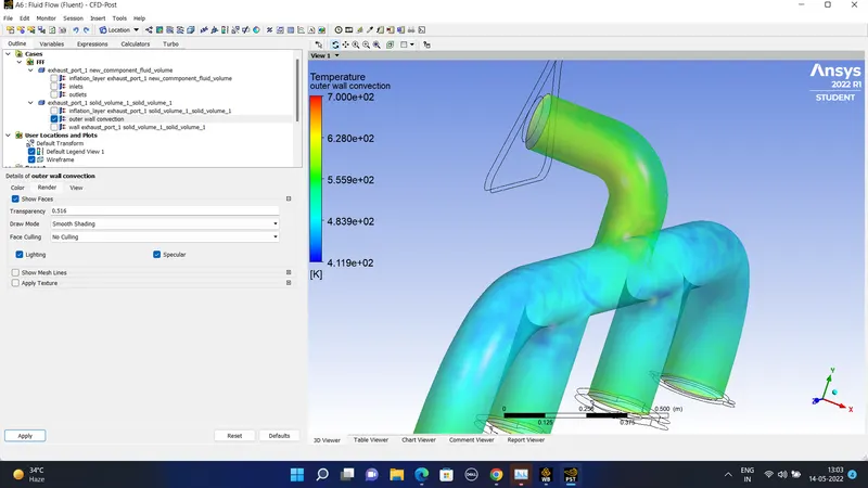
Contours of static temperature

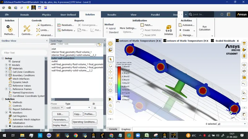
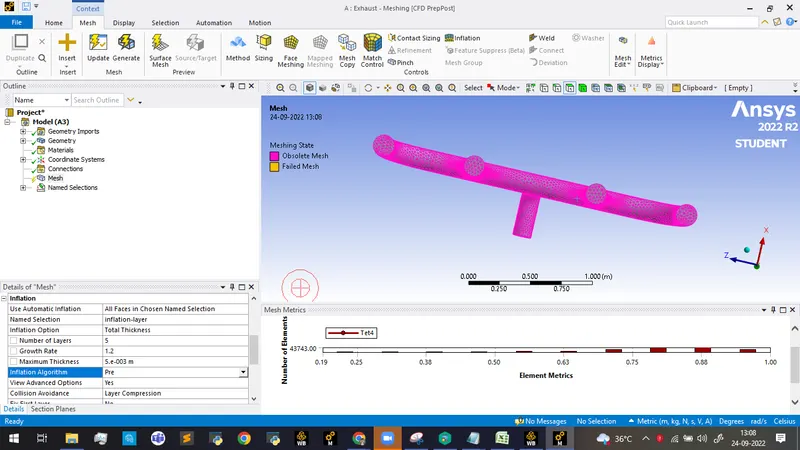
Refining the mesh by creating an inflation layer with a total thickness of 5 mm.

AIM of the project- To perform the steady-state conjugate heat transfer simulation on the exhaust port when the air is coming at the inlet at a speed of 5m/sec.

The objective of the project is to mainly focus on the following-

1) Definition of the Conjugate heat transfer analysis- Conjugate heat transfer analysis is based on the mathematical structure problem which describes the heat transfer between the body and the fluid flowing over or inside it as a result of interaction between two objects. At the matching interface, the details are provided for temperature distribution and heat flux along the interface eliminating the need of calculating the heat transfer coefficient.

CHT analysis type allows for the simulation of the heat transfer between the solid and liquid domains by exchanging thermal energy at the interface between them. The simulation of the heat exchangers, cooling of the electronic equipment, and general-purpose cooling and heating system. In the case of CHT that is being done in this project, we have the convection mode of heat transfer between the fluid and the solid aluminum wall of the exhaust pipe and then the conduction mode of heat transfer is followed within the wall of the exhaust pipe wall.

3) Solving and modelling approach-

1) The exhaust pipe was modeled in the space claim.

2) The exhaust port is a three dimensional model containing four inlets and one outlet. Despite having the isothermal boundary condition and a uniform flow rate at the four inlets the model can not be cut into two halves to save computational power. Therefore the whole model needs to be discretized it is also called as space discretization.

3) CHT analysis requires the both the solid and the liquid volume under consideration spaceclaim gives an option of volume extract for selecting the edges for fluid volume.

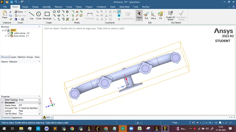
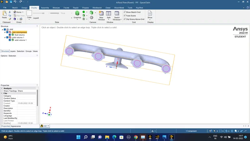
4) Both the solid component and the liquid component are copied into one component.

5) Share topology is created.

6) Spaceclaim gives an option for share coincident topology when share coincident topology is selected and executed. The , mesh from the fluid volume and the solid volume are said to be conformal with each other which is a requirement for the CHT analysis.

7) The exhaust port is loaded with the proper geometry and it is then si9mulated for the baseline computer generated mesh and in the next half we are going to be when we are going to use the refined mesh using the inflation layer and the element size is to be updated to 25 mm and hence a finer result is obtained.

8) The named selection is created like the inlet one, outlet one, and the outlet and the wall-convection is created to study thye effect of convection from the fluid to the wall and from the wall the heat is dissipated by the heat conduction method.

The geometry in the spaceclaim-

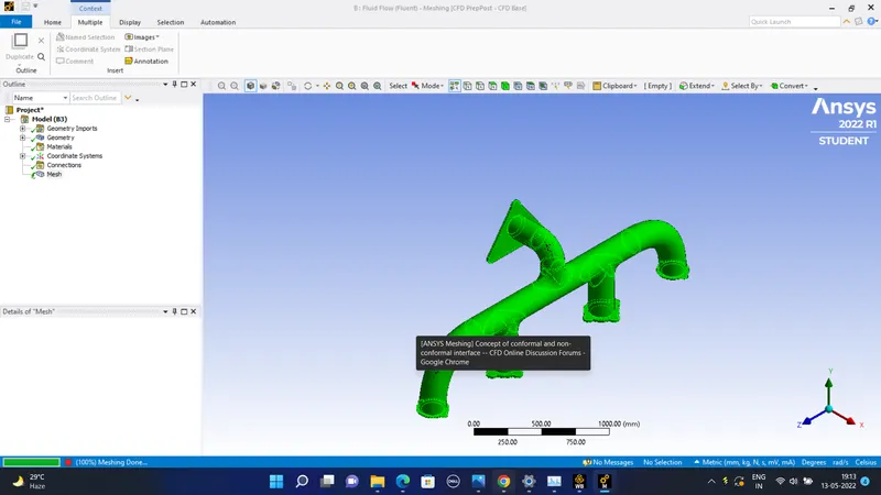
Inside the spaceclaim the extra edges were found in the geometry that was provided we have to removed by the option of prepare and the six edges were removed.

2) Then the volume extraction tool is used for the five edges and the volume and the process of fluid volume extraction is used for the edges to create the fluid volume.

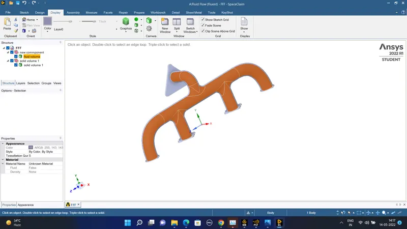
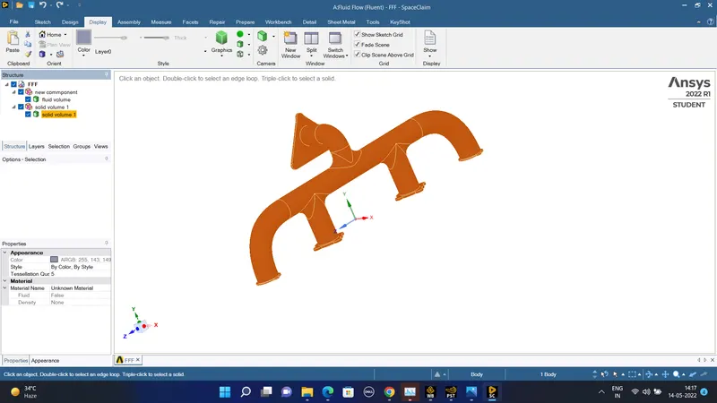
The solid volume is created -

The solid and the fluid volume is created in the new component and it is kept inside it-

The baseline mesh that is created due to the original geometry with less modifications-

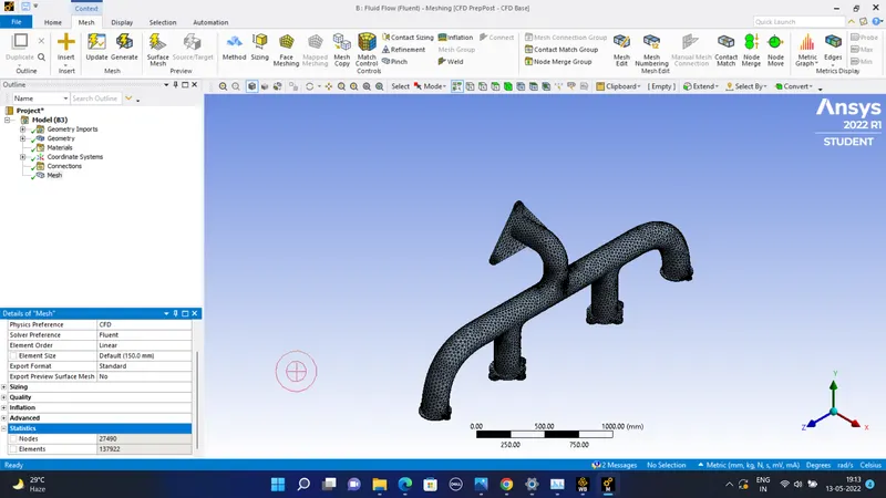
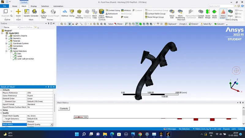
Mesh quality is that it conatins more than 1lakh 30 thousands elements and the nodes are of more than 27 thousand nodes.

#) Then it is imported in the fluent solver to perform the CHT flow heat transfer analysis-

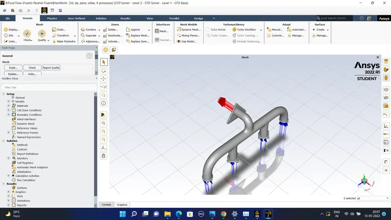
The following inputs of the varibale is made into the following velocity v = 5 m/sec at the inlet with the temperature of the fluid to be 700 kelvins. The boundary condition applied at the inlet is of velocity inlet.

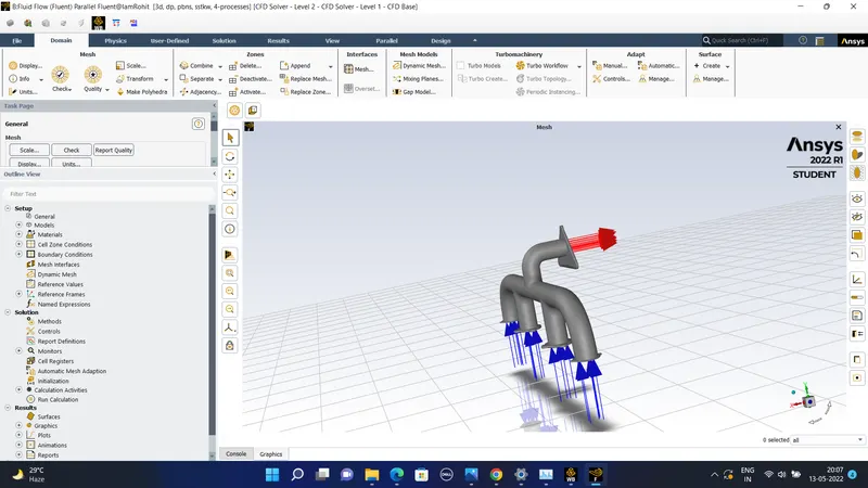
The red arrow indicates the outlet the boundary condition is of the pressure outlet type-

#) The third boundary condition is applied to the outer wall with a heat transfer coefficient of k = 20 w/m^2-k .

The steady state pressure based solver is used with the SIMPLE algorithm and the turbulence model that is used of the k- epsilon turbulence model is used with the outlet Gauge pressure = 0 pa and the energy equation is turned on.

material properties-

Fluid -

Fluid name = air.

Density = 1.225 kg/m^3

Specific heat = 1006.43 J/kg-k

thermal conductivity = 0.0242 w/m-k

viscosity = 1.789e-5 kg/m-sec.

Solid -

the solid material is of aluminum

Specific heat = 871 J/kg-k .

Thermal conductivity = 20 w/M-k

The temperature contours-

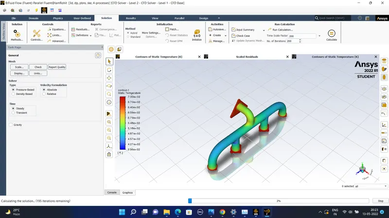
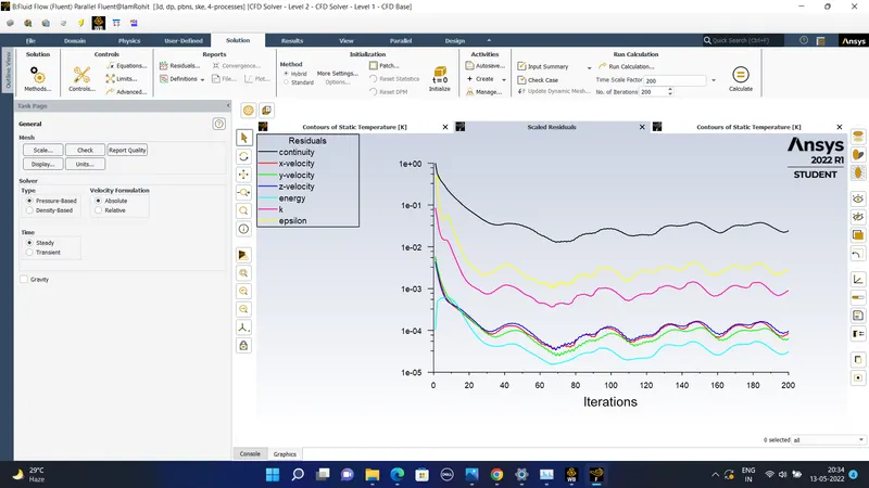
Since the residuals have dropped below the 1e-4 and between 1e-5 we get the solutions as converged.

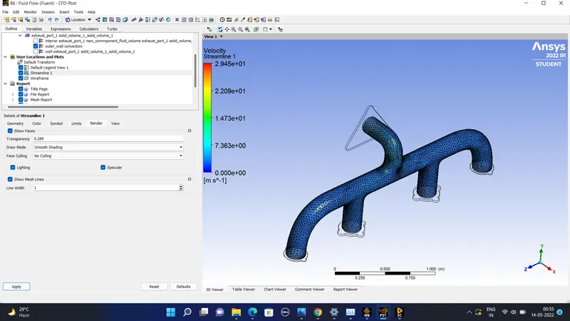
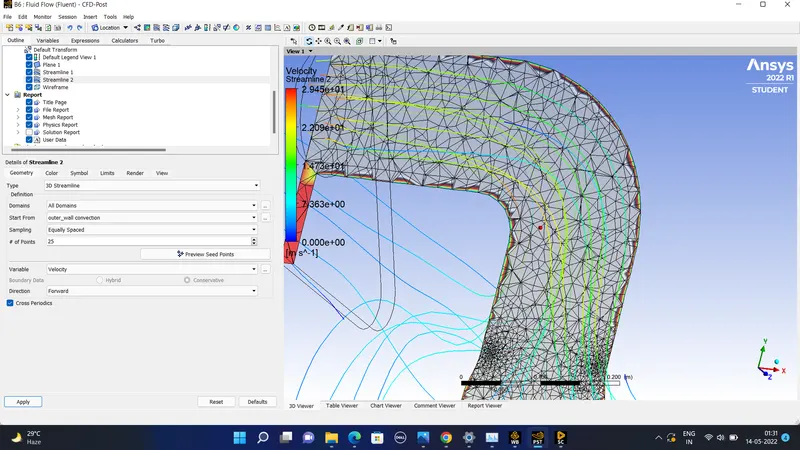
The streamlines of velocity-

case 2 ) In these the inflation layers are added and the element size of the solid surface mesh is also reduced further to 10 mm size-

The Inflation layer is added to the geometry 6 layers are added

Growth rate = 1.2

Number of inflation layers = 6

First layer thickness = 0.0514 mm

captured curvature is set to yes.

The mesh looks like this form-

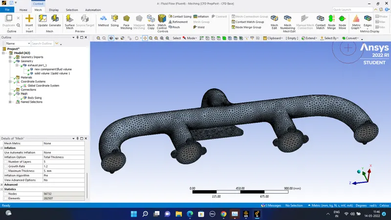
The number of elements for this mesh is of 282507

Using the same solver and the same boundary band initial conditions we get the following outcomes-

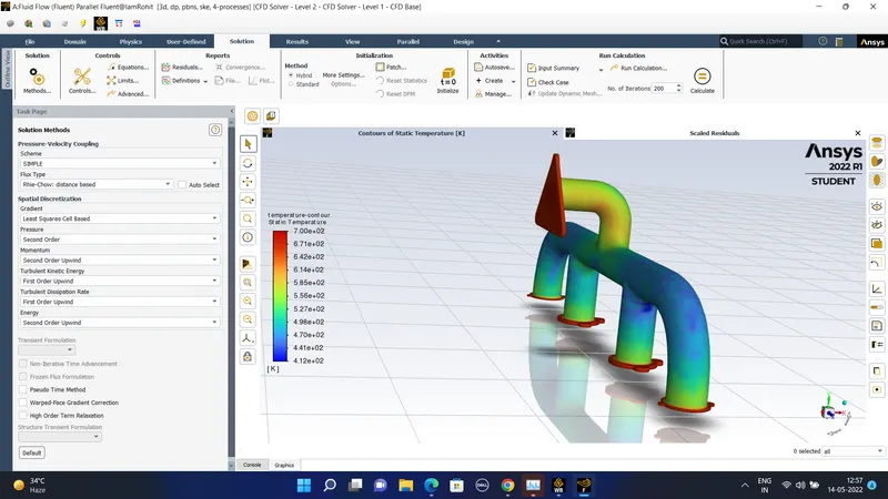
The plot of the residuals-

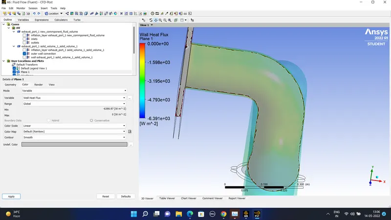
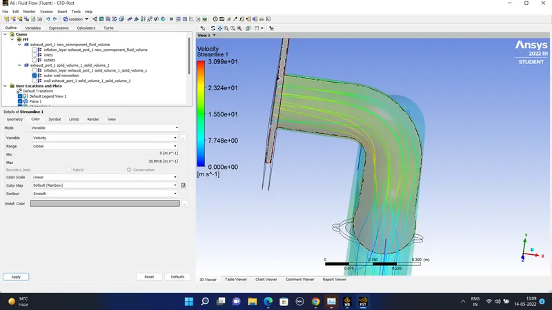
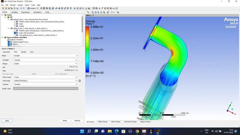
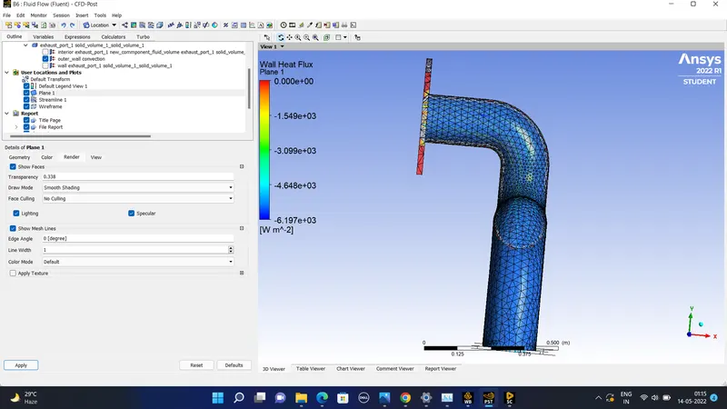
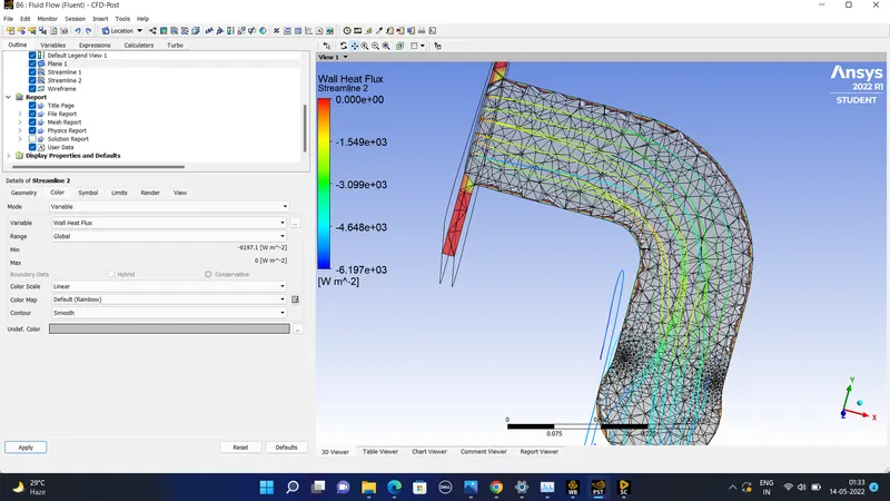
The point of the localized heat flux source is maximum at the turning point which denotes that the same point of maximum velocity will be the point of the maximum heat transfer or the max heat flux this is evident from the contour obtained.

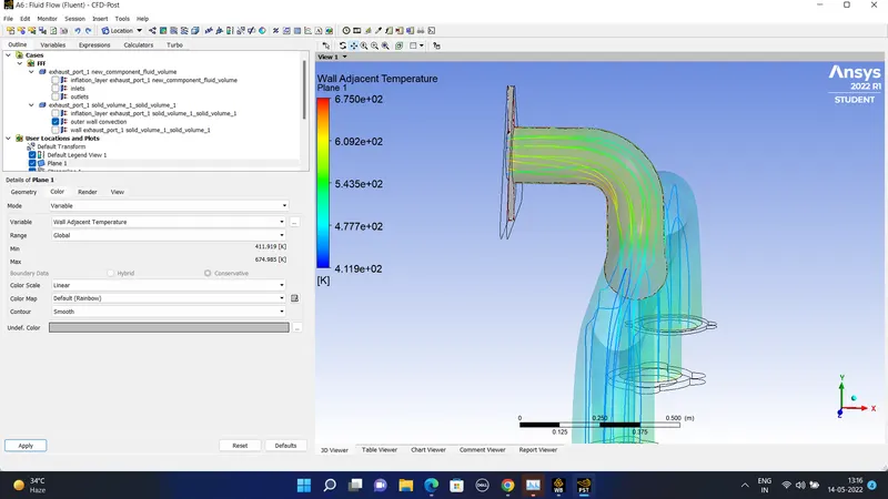
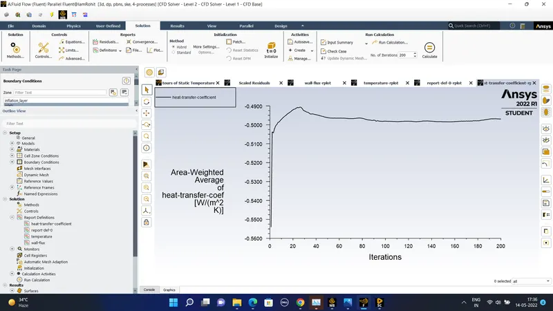
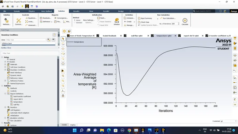
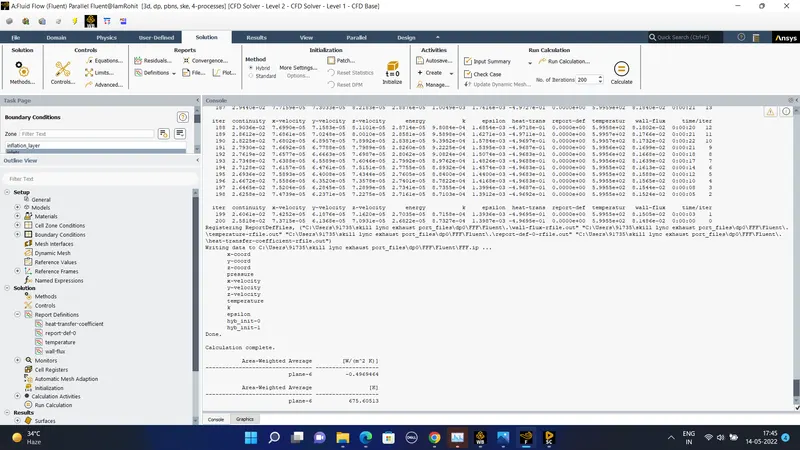
This shows the area weighted average heat transfer coefficient = 0.469 w/m^2k. and the area weighted average of the temperature = 475.40k

In the analysis, the heat transfer coefficient obtained is of h = 20.66 w/m^2-k

#) Analytical solution-

The Reynolds number of the flow is of Re = 56867.66 considering the flow velocity = 5 m/sec

By using the Dittus Bolter heat transfer coefficient relation in natural turbulent flowe the Diltus Bolter HT coefficient is determined by the Nusselt number which is related by the formula of

Nu(D) = 0.023* Re^(4/5)*pr^n here n = 0.3 . D = diamter of the pipe = characteristics length = 0.166 m

the prandtl number is of the following

pr = mu*cp/k here mu = 1.789*10^-5 cp = 1006.43 J/kg-k and k = thermal conductivity = 0.0242 w/mk

pr = (1.789*10^-5*20)/0.0242 = 0.744

the Nusselt number is calculated as NUd = 0.023*56867.66^(4/5)*0.744^0.3 = 131.792

Nud = hD/k = 131.792 = h*0.166/0.0242

so h = 19.52 w/m^2k.

Conclusions-

1) Here we find the theoretical value and the computational value of the thermal specific heat transfer coefficient to be = 19.52 so the value is really close to the value of h in the computational way which is = 20 w/m^2k.

2) When we are using the finer grid by applying the inflation layer and reducing the element size to be nearly 10 mm we are getting the result with much less deviation.

3) The value of the heat transfer coefficient is located in the call adjacent to the wall which allows allows us to choose the value of y+ = 1 for the turbulence model.

4) The presence of the boundary layer is quite visible near the inlet of the wall where the velocity near the wall are to be close to be 0 to be the zero slip boundary condition so the viscous force is dominant near the inlet but near the outlet the velocity is the highest so giving the highest Reynolds number.

5) The velocity at the outlet is high than in the inlet this can be attributed to one outlet and the four inlets.

6) The value of the y+ is maintained in the range of 1 for the turbulence model . This is validated with the analytical solution which comes out to be near to it. The value of the heat transfer coefficien is found out to be 20.45 w/m^2k. which is close to the analytical value.