Week 1- Mixing Tee
Introduction
Mixing tees—in which two fluid streams with different physical and/or chemical properties mix—are widely used in the petrochemical industry. When there is a large temperature difference between two streams, large metal temperature fluctuations can occur in the region where the two streams meet if proper design steps are not taken. The temperature fluctuations in the metal can lead to thermal fatigue of the pressure boundary piping. If through-wall cracking occurs, the fluid may leak, possibly causing a fire and damage. Therefore, it is imperative to ensure that the piping system can withstand the temperature fluctuations. Options can include improving the mixing of the two streams to reduce the temperature fluctuations through redesign of the piping system such that the momentum ratio of the two fluid streams is favorable to rapid mixing, or installing devices that protect the pressure boundary piping (e.g., injection quills or thermal sleeves in the region where the temperature fluctuations are higher than a thermal fatigue threshold). This region includes the T-junction and a length of differing main pipe diameters downstream from the T-junction. For thermal sleeves, different approaches exist to determine the needed sleeve length, which are briefly discussed in this article.
Empirical correlations in the literature may be used to estimate mixing effectiveness or the uniformity of the fluid concentrations over the pipe cross-section downstream from the T-junction, whereby the length of the pipe that needs protection can be determined. However, these correlations were developed based on experiments typically using air or water as working fluids and a chemical agent as the tracer to indicate the mixing uniformity. The temperature differences between the two fluid streams in these experiments were usually small. Therefore, these correlations should be used with caution when the actual fluid conditions are well outside of the range in which the correlations were developed.
Computational fluid dynamics (CFD) modeling, such as wall-resolved large eddy simulation (LES), can provide accurate predictions of the mixing behavior—including velocity, concentration and temperature fields—in a mixing tee. Therefore, the variations of the transient fluid temperature can be used to identify a location in the main pipe downstream of the tee, after which the circumferential maximum temperature difference is less than the thermal fatigue threshold.
Advanced CFD modeling can predict the fluid temperature fluctuations at the mix point, as well as characterize the corresponding temperature variations in the pipe wall. Specifically, LES is required to capture the time-varying turbulent behavior at the mixing point, which is significantly more time- and resource-intensive than traditional two-parameter (e.g., k-ε and k-π) Reynolds-averaged Navier-Stokes (RANS) simulation, which is the workhorse of most industrial CFD simulations.
Aim
The aim is to set up steady-state simulations to compare the mixing effectiveness when hot inlet temperature is 360C & the Cold inlet is at 190C.
To use the k-epsilon and k-omega SST model for the first case and based on your judgment use the more suitable model for further cases along with specifying the reason for choosing a suitable model is compulsory.
- Case 1
- Short mixing tee with a hot inlet velocity of 3m/s.
- Momentum ratio of 2, 4.
- Case 2
- Long mixing tee with a hot inlet velocity of 3m/s.
- Momentum ratio of 2, 4.
Solution Case setup
The fluent is opned with double precision and display mesh after reading checked along with choosing a parallel solver upto 4 solver processes.
In the fluid flow fluent solver window the solution case setup is specifed. After importing the mesh it is checked initially and the following steps are performed.
1. The temperature unit is set to degrees Celsisus.
2. Within the physics tab, the energy equation is enabled and in the viscous model k-epsilon or k-omega SST model is chosen. In the boundaries section the velocity and temperature for both the hot and cold inlets are specified. The temperatures at the hot and cold inlets are 36 and 19 respectively. The velocity of fluid at hot inlet is 3 m/s and at cold inlet is 6 m/s , for momentum ratio 2 . The velocity at cold inlet is 12 m/s when the momentum ratio is 4. Momentum ratio = velocity at cold inlet / velocity at hot inlet.
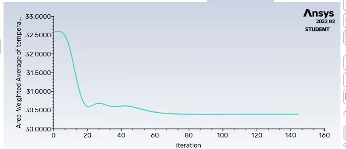
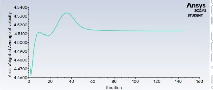
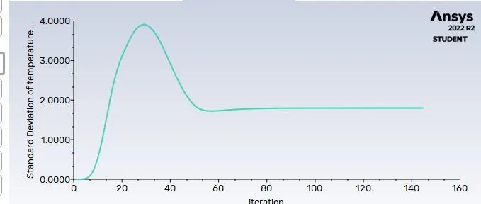
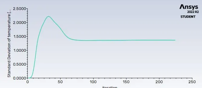
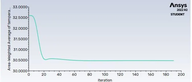
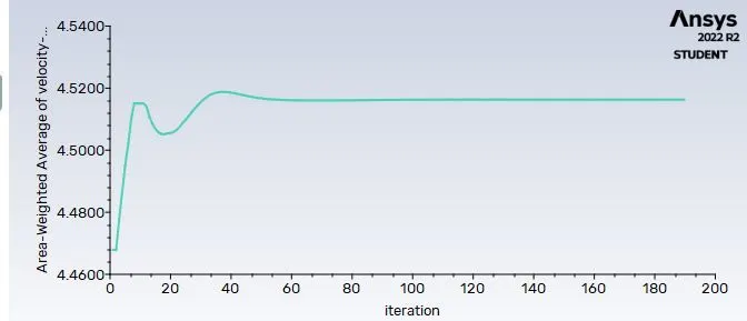
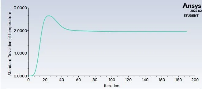
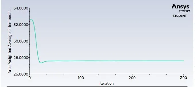
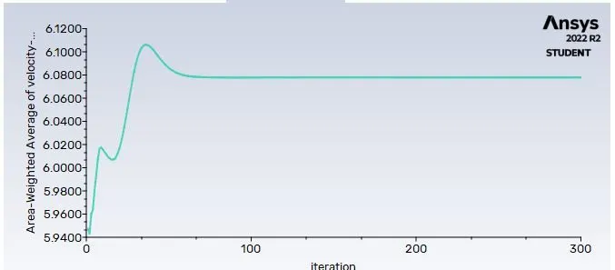
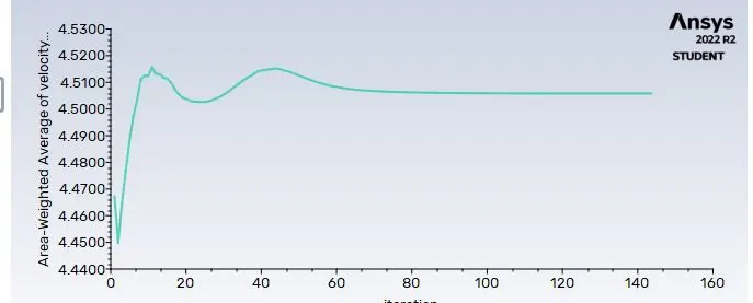
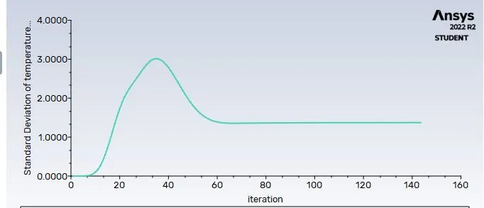
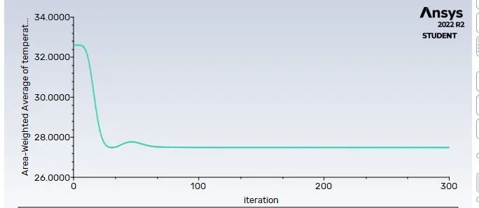
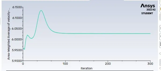
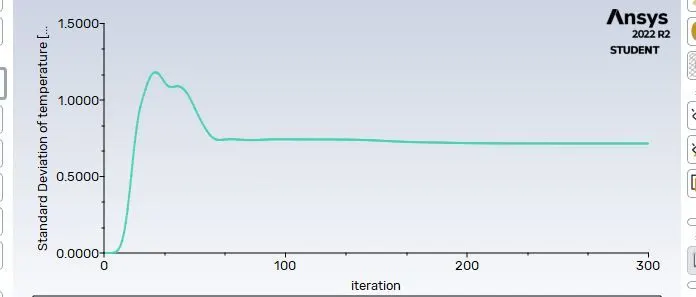
3. The solution plots are then defined by creating new plot definitions such as area weighted average pf temperature and velocity along with standard deviation of temperature at the outlet.
4. The hybrid initialization is performed at t = 0 after specifying the convergence criteria to check if the criterion is satisfied after which the case check can be done to get recommendations.
5. The solution is calculated after specifying hte number of iterations(in this case 300).
k-Epsilon model
Intially the k-Epsilon realizable model with enhanced near wall is used to determine flow through a mixing tee.
- Case 1
- Short mixing tee with a hot inlet velocity of 3m/s.
- Momentum ratio of 2, 4.
Short Tee Geometry
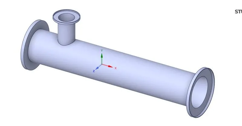
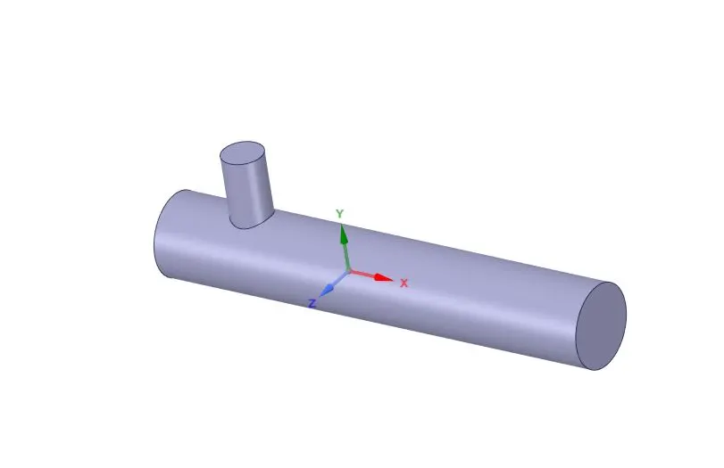
After extracting the voulme and supressing physics for this solid model the geometry becomes,
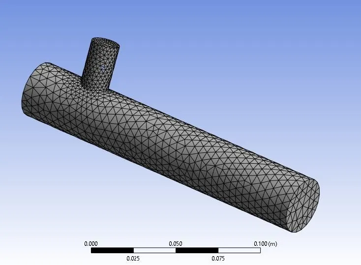
Baseline mesh conditions
The element size for meshing is not specified and the mesh is generated after specifying the named selections i.e., inlet-x,inlet-y,outlet and walls.
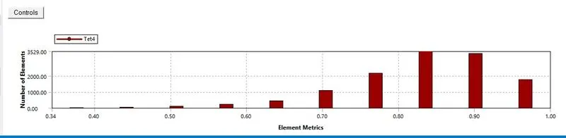
Mesh Metrics
A mesh element metric that identifies the quality of mesh was employed and it can be seen that the elements of the lowest quality are minimal. Most of the elements have quality in the range of 0.7-1. Hence, the mesh is of acceptable quality.
Output plots and images
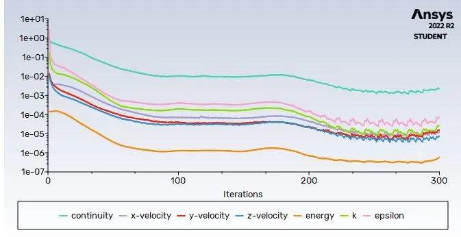
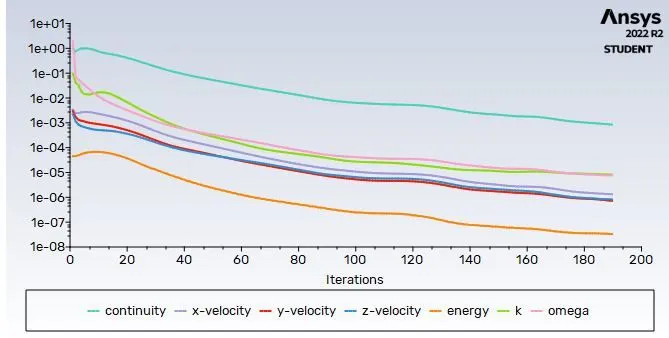
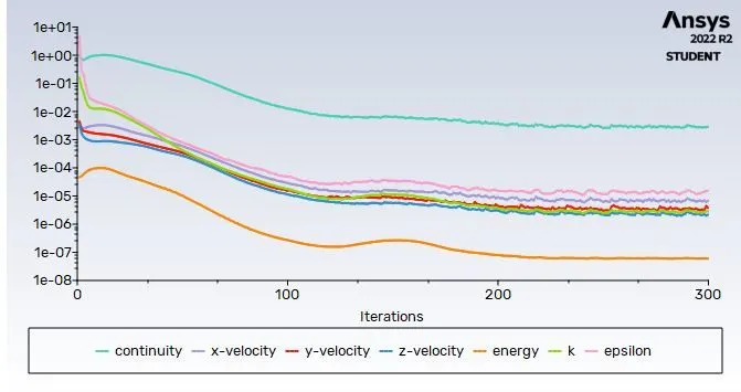
Scaled Residuals
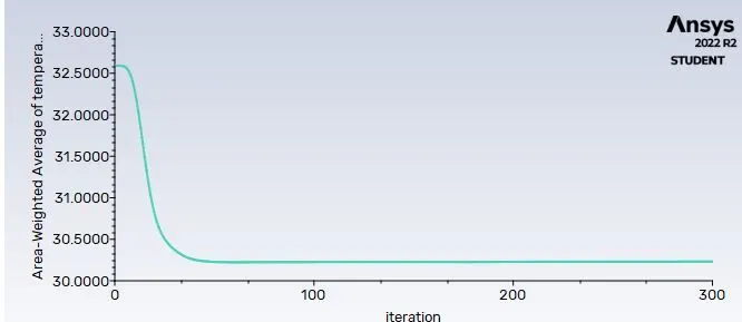
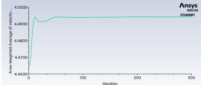
Area weighted average of temperature and velocity
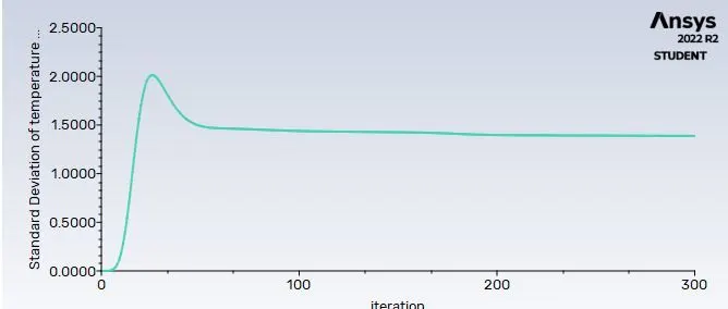
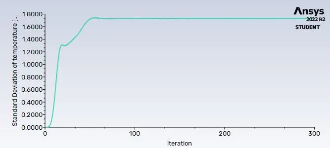
Standard deviation of temperature
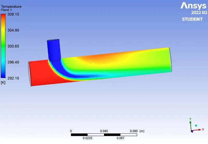
Temperature distribution
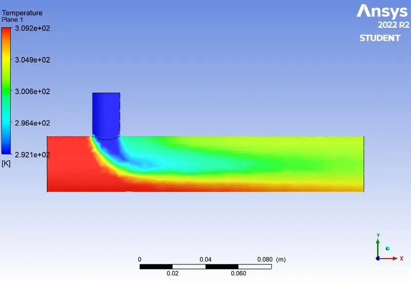
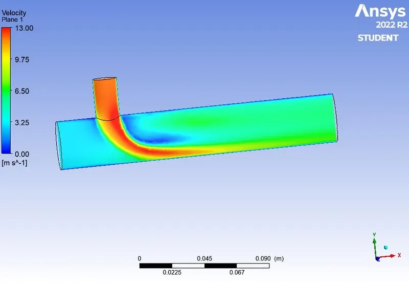
Velocity distribution
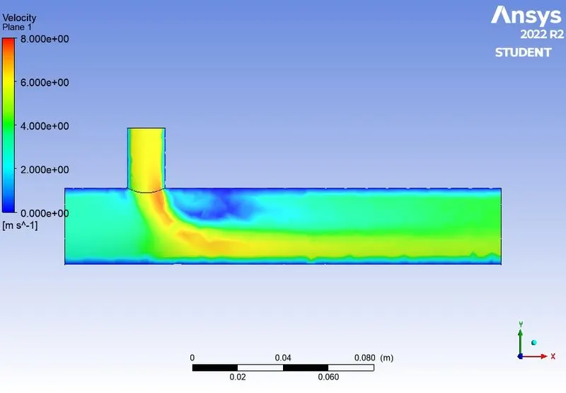
Since the mesh is not refined and fine, the mesh is refined by specifying an element size to obtain a finer mesh and hence generate a smooth output of distributions.
Refined mesh
The element sizing is specifed as 0.0011 m for the short tee case.
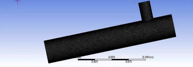

A mesh element metric that identifies the quality of mesh was employed and it can be seen that the elements of the lowest quality are minimal. Most of the elements have quality in the range of 0.7-1. Hence, the mesh is of acceptable quality.
Momentum ratio 2
Output plots and images
Scaled Residuals
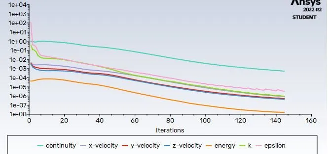
Area weighted average of temperature and velocity
Standard deviation of temperature
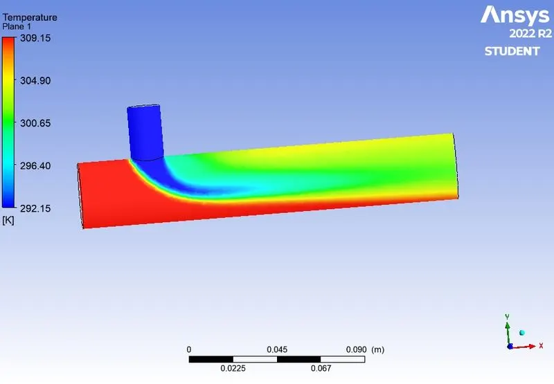
Temperature distribution
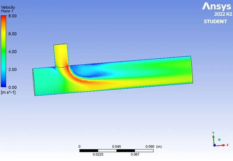
Velocity distribution
Momentum ratio 4
Output plots and images
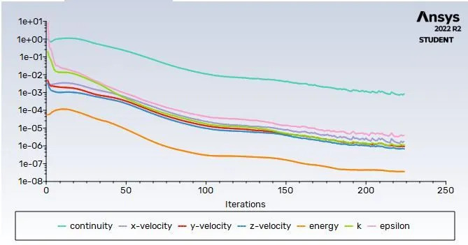
Scaled Residuals
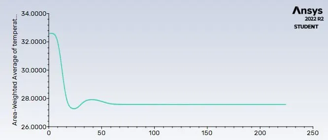
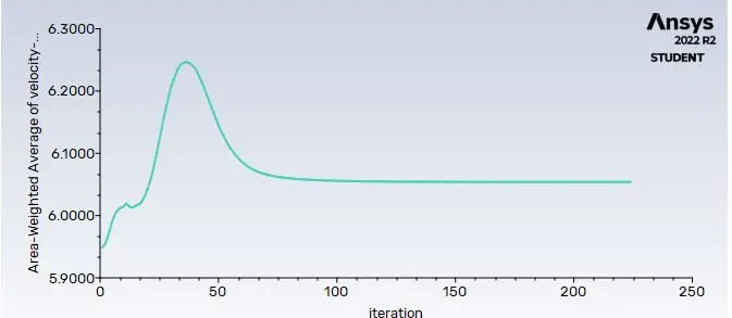
Area weighted average of temperature and velocity
Standard deviation of temperature
Temperature distribution
Velocity distribution
k-omega SST model
Momentum ratio 2
Output plots and images
Scaled Residuals
Area weighted average of temperature and velocity
Standard deviation of temperature
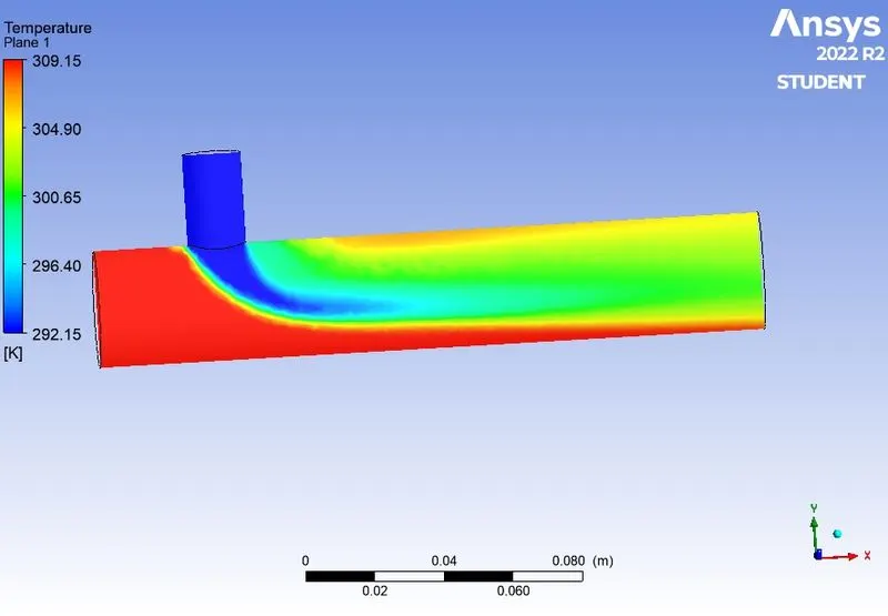
Temperature distribution
Velocity distribution
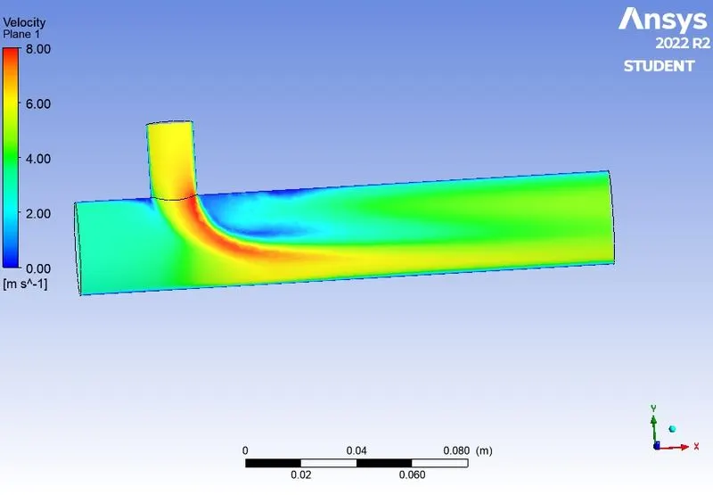
Momentum ratio 4
Output plots and images
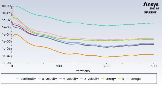
Scaled Residuals
Area weighted average of temperature and velocity
Standard deviation of temperature
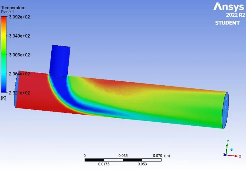
Temperature distribution
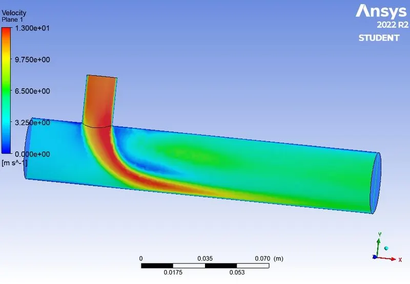
 Velocity distribution
From the above plots it can be inferred that,
1. The k-epsilon approach attains a quicker convergence than the the k-omega SST approach.
2.The k-ε model has been tailored specifically for planar shear layers and recirculating flows. This model is the most widely used and validated turbulence model with applications ranging from industrial to environmental flows, which explains its popularity. It is usually useful for free-shear layer flows with relatively small pressure gradients as well as in confined flows where the Reynolds shear stresses are most important.It can also be stated as the simplest turbulence model for which only initial and/or boundary conditions needs to be supplied.However it is more expensive in terms of memory than the mixing length model as it requires two extra PDEs. This model would be an inappropriate choice for problems such as inlets and compressors as accuracy has been shown experimentally to be reduced for flows containing large adverse pressure gradients. The k-ε model also performs poorly in a variety of important cases such as unconfined flows, curved boundary layers, rotating flows and flows in non-circular ducts.
3. Realizable k-ε Model: An immediate benefit of the realizable k-ɛ model is that it provides improved predictions for the spreading rate of both planar and round jets. It also exhibits superior performance for flows involving rotation, boundary layers under strong adverse pressure gradients, separation, and recirculation. In virtually every measure of comparison, Realizable k-ɛ demonstrates a superior ability to capture the mean flow of the complex structures.
4. In computational fluid dynamics, the k–omega (k–ω) turbulence model is a common two-equation turbulence model that is used as an approximation for the Reynolds-averaged Navier–Stokes equations (RANS equations). The model attempts to predict turbulence by two partial differential equations for two variables, k and ω, with the first variable being the turbulence kinetic energy (k) while the second (ω) is the specific rate of dissipation (of the turbulence kinetic energy k into internal thermal energy).
5. As k-epsilon model attains faster convergence than k-omega SST model ,the k-epsilon approach is used for further calculations.
Case 2
- Long mixing tee with a hot inlet velocity of 3m/s.
- Momentum ratio of 2, 4.
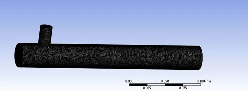
Long tee geometry
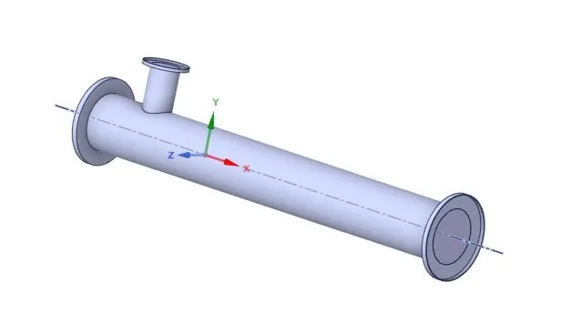
After extracting the voulme and supressing physics for this solid model the geometry becomes,
Refined mesh
The element sizing is specifed as 0.0013 m for the short tee case.
Mesh metrics
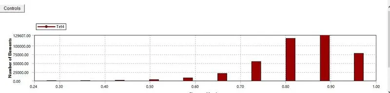
A mesh element metric that identifies the quality of mesh was employed and it can be seen that the elements of the lowest quality are minimal. Most of the elements have quality in the range of 0.7-1. Hence, the mesh is of acceptable quality.
Momentum ratio 2
Output plots and images
Scaled Residuals
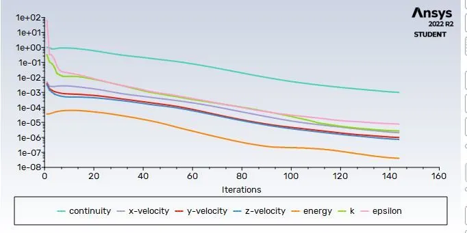
Area weighted average of temperature and velocity
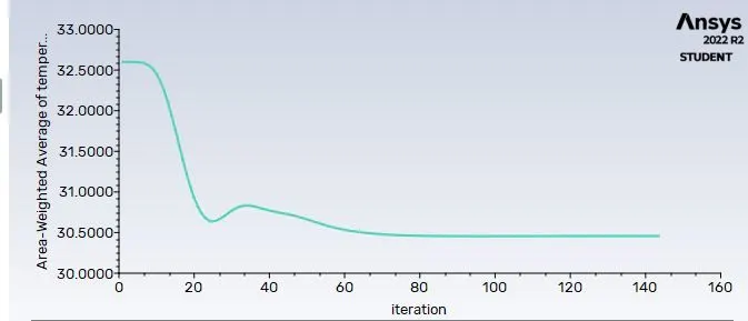
Standard deviation of temperature
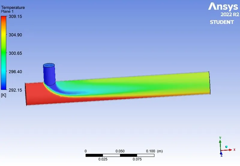
Temperature distribution
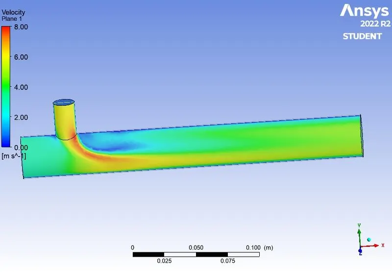
Velocity distribution
Momentum ratio 4
Output plots and images
Scaled Residuals
Area weighted average of temperature and velocity
Standard deviation of temperature
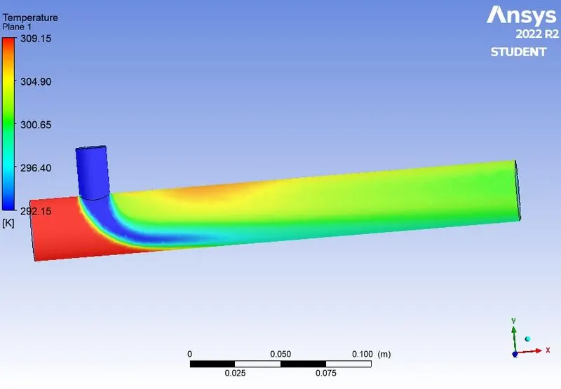
Temperature distribution
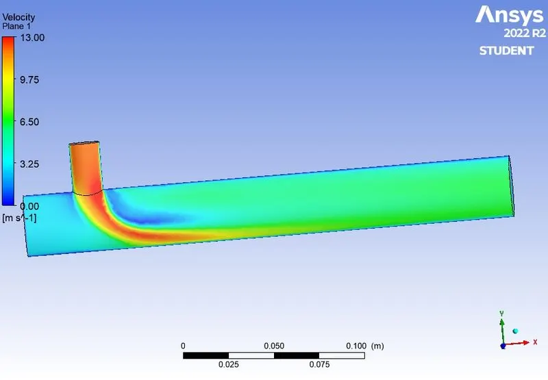
Velocity distribution
| Case | Cell count | Average outlet temperature(K) | No of iterations for convergence |
| Short tee- Momentum ration 2 | 457846 | 303.459 | 148 |
| Short tee- Momentum ration 4 | 457846 | 300.699 | 228 |
| Long tee- Momentum ration 2 | 412867 | 303.549 | 148 |
| Long tee- Momentum ration 4 | 412867 | 300.639 | 298 |
CONCLUSION:
- As seen in the Case-1-a and Case-1-b, the temperature at the outlet drops down significantly due to high velocity of cold air from the inlet. This is possible due to the turbulent mixing at the tee joint between hot air and cold air because of the high velocity of cold air., which is not possible in case of low-velocity cold air.
- The temperature contour at the outlet for short tee cases shows that some of the high temperatures flow sips through without properly mixing with the flow. Whereas, in the temperature contour of long tee cases, the high temperatures flow thoroughly mixes with the rest of the flow.