Week 3.5 - Deriving 4th order approximation of a 2nd order derivative using Taylor Table method

Taylor Series

In mathematics, the Taylor series of a function is an infinite sum of terms that are expressed in terms of the function's derivatives at a single point. For most common functions, the function and the sum of its Taylor series are equal near this point. Taylor series are named after Brook Taylor, who introduced them in 1715. If 0 is the point where the derivatives are considered, a Taylor series is also called a Maclaurin series, after Colin Maclaurin, who made extensive use of this special case of Taylor series in the mid 1700s.

The partial sum formed by the first n + 1 terms of a Taylor series is a polynomial of degree n that is called the nth Taylor polynomial of the function. Taylor polynomials are approximations of a function, which become generally better as n increases. Taylor's theorem gives quantitative estimates on the error introduced by the use of such approximations. If the Taylor series of a function is convergent, its sum is the limit of the infinite sequence of the Taylor polynomials. A function may differ from the sum of its Taylor series, even if its Taylor series is convergent. A function is analytic at a point x if it is equal to the sum of its Taylor series in some open interval (or open disk in the complex plane) containing x. This implies that the function is analytic at every point of the interval.

Taylor Tables

Taylor's series expansion of functions about a fixed point provides a means for constructing finite-difference operator of any order. A simple and straight forward way to carry out this is to construct Taylor's table. The table is constructed to simplify the algebra and reduce the operation time.

Main Script

clear all
close all
clc

%Defining the input parameters

x = pi/4;
dx = linspace(pi/4,pi/4000,100);

f = @(x) exp(x).*cos(x);

 %Calculating the errors
  for i = 1:length(dx)
  
     c_e(i) = cd_a(x,dx(i),f);
     rs_e(i) = rs_a(x,dx(i),f);
     ls_e(i) = ls_a(x,dx(i));
 
 end

%Plotting the values of dx vs errors for each approximation type

 figure(1)
   loglog(dx,c_e,'color','#FFA500','linewidth',3)
   hold on
   loglog(dx,rs_e,'color','r','linewidth',3)
   hold on
   loglog(dx,ls_e,'g','linewidth',2)
   grid
   xlabel('dx')
   ylabel('Absolute error')
   legend('Central error', 'Right skewed error', 'Left skewed error','Location','eastoutside')
   title('Plot of dx vs errors')

Function Scripts

Central difference scheme

%Function for central differencing scheme 

function c = cd_a(x, dx, f)
  
  %f(x) = exp(x)*cos(x)
  %Analytical derivative = f'(x) = -2*exp(x)*sin(x) 
  
  analytical_derivative = -2*exp(x)*sin(x);
  
  % numerical derivative
  %fourth order central differencing approximation
  %calcuation of arbitrary constants (a, b, c, d, e) for numerical derivative
syms a b c d e
e_1 = a + b + c + d + e == 0;
e_2 = -2*a - b + 0 + d + 2*e == 0;
e_3 = 2*a + b/2 + 0 + d/2 + 2*e == 1;
e_4 = -8*a/6 - b/6 + 0 + d/6 + 8*e/6 == 0;
e_5 = 16*a/24 + b/24 + 0 + d/24 + 16*e/24 == 0;

%Solving Equations to calculate constants
X = solve([e_1, e_2, e_3, e_4, e_5], [a, b, c, d, e]);

%Extracting values of constants from solution
a = X.a;
b = X.b;
c = X.c;
d = X.d;
e = X.e;
  
central_differencing = (a*f(x-2*dx) + b*f(x-dx)+ c*f(x) +d*f(x+dx) + e*f(x+2*dx))/dx^2;
  
%  central_differencing = ((a*exp(x-(2*dx))*cos(x-(2*dx))) + (b*exp(x-dx)*cos(x-dx))+ (c*exp(x)*cos(x)) + (d*exp(x+dx)*cos(x+dx)) + (e*exp(x+(2*dx))*cos(x+(2*dx))))/(dx^2);
 
 %output
     c = abs(central_differencing - analytical_derivative);

end

Skewed right sided difference scheme

%Function for Skewed right sided differencing scheme 

function r = rs_a(x, dx,f)
  
  %f(x) = exp(x)*cos(x) = exp(x)-sin(x) + expxcosx =
  %-expxsinx-expxcosx+expxcosx - expxsinx
  %Analytical derivative = f''(x) = -2*exp(x)*sin(x) 
  
  analytical_derivative = -2*exp(x)*sin(x);
  
%calcuation of arbitrary constants (a, b, c, d, e) for numerical derivative
syms a b c d e h
e_1 = a + b + c + d + e + h == 0;
e_2 = b + 2*c + 3*d + 4*e + 5*h == 0;
e_3 = b/2 + 4*c/2 + 9*d/2 + 16*e/2 +25 *h/2 == 1;
e_4 = b/6 + 8*c/6 + 27*d/6 + 64*e/6 +125*h/6 == 0;
e_5 = b/24 + 16*c/24 + 81*d/24 + 256*e/24 + 625 * h/24 == 0;
e_6 = b/120 + 32*c/120 + 243*d/120 + 1024*e/120 + 3125*h/120 == 0;

%Solving Equations to calculate constants
X = solve([e_1, e_2, e_3, e_4, e_5, e_6], [a, b, c, d, e, h]);

%Extracting values of constants from solution
a = X.a;
b = X.b;
c = X.c;
d = X.d;
e = X.e;
h = X.h;
  
%  rightskewed_differencing = ((a*exp(x)*cos(x)) + (b*exp(x+dx)*cos(x+dx))+ (c*exp(x+(2*dx))*cos(x+(2*dx))) + (d*exp(x+(3*dx))*cos(x+(3*dx))) + (e*exp(x+(4*dx))*cos(x+(4*dx)+(h*exp(x+(5*dx))*cos(x+(5*dx))))/(dx^2);

 rightskewed_differencing = (a*f(x) + b*f(x+dx)+ c*f(x+2*dx) +d*f(x+3*dx) + e*f(x+4*dx) + h*f(x+5*dx))/dx^2;
  

 
 %output
     r = abs(rightskewed_differencing - analytical_derivative);

end

Skewed left sided difference scheme

%Function for Skewed left sided differencing scheme 

function l = ls_a(x, dx)
  
  %f(x) = exp(x)*cos(x)
  %Analytical derivative = f'(x) = -2*exp(x)*sin(x) 
  
  analytical_derivative = -2*exp(x)*sin(x);
  
 %calcuation of arbitrary constants (a, b, c, d, e) for numerical derivative
syms a b c d e h
e_1 = a + b + c + d + e + h == 0;
e_2 = - e  - 3*c - 2*d -4*b -5*a == 0;
e_3 = e/2 + 9*c/2 + 4*d/2 + 16*b/2  + 25*a/2 == 1;
e_4 = -e/6 -27*c/6 - 8*d/6 -64*b/6 - 125*a/6 == 0;
e_5 =  e/24 + 81*c/24 + 16*d/24 + 256*b/24 + 625*a/24 == 0;
e_6 = - e/120- 243*c/120 - 32*d/120  -1024*b/120- 3125*a/120 == 0;

%Solving Equations to calculate constants
X = solve([e_1, e_2, e_3, e_4, e_5, e_6], [a, b, c, d, e, h]);

%Extracting values of constants from solution
a = X.a;
b = X.b;
c = X.c;
d = X.d;
e = X.e;
h = X.h;
 leftskewed_differencing = ((h*exp(x)*cos(x))+ (e*exp(x-dx)*cos(x-dx))+ (d*exp(x-(2*dx))*cos(x-(2*dx))) + (c*exp(x-(3*dx))*cos(x-(3*dx))) + (b*exp(x-(4*dx))*cos(x-(4*dx))) + (a*exp(x-(5*dx))*cos(x-(5*dx))))/(dx^2);
  
 %leftskewed_differencing = ( a*f(x) + b*f(x-dx)+ c*f(x-2*dx) +d*f(x-3*dx) + e*f(x-4*dx) + h*f(x-5*dx))/dx^2;
  

 %output
     l = abs(leftskewed_differencing - analytical_derivative);

end

Output plot of dx vs errors

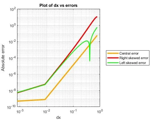
Script Explanantion

1. Define the input parameters x and dx. As dx is defined over a range of values the linspace function is used.

2. The function exp(x)*cosx is defined and assigned to a variable f. It is mentioned using the syntax @x so that matlab replaces x at all positions in the code by expx*(cosx)

3.For calculating the errors over a range of values a for loop is used in which the values ranges from 1 to the length of dx and the error values for central difference,skwed right side and skewed left side difference schemes are calculated.

4. The erros are plotted in a plot of dx vs errors with dx on the x-axis and absolute errors on y-axis. The plot is provided with legends and a proper title along with different colours for each scheme.This facilitates in a neat plot and aids in clear understanding.

5. The function scripts for each scheme is defined separately. Exact inpiut and output arguments must be defined so that matlab does not return any errors when the function is called into the main program. The function script must be given a name of specified format and saved in the same folder as the main script.

6. The second derivative for the function exp(x)*cos x is determined and assigned to a separate variable. The second order deriavative is obtained by derivating the function twice.

7.The equations are derived by using the values from the Taylor Table. The arbitarary constants for each numerical derivative are calculated . The value of X is obtained by using the solve function to solve the equations.

8. The values of the constants are extracted from the solution.The values for the different schemes are then calculated by using the respective constants and formula for each scheme.

9. The error is obtained by calculating the difference between the values for each scheme and the analytical derivative.

Conclusion:- By observing the plot we can conclude the following observations which are as follows

• Skewed right gives maximum error or in other words we can say that its unstable as compared to other scheme.
• Central difference gives lowest error or in other words we can say that its stable as compared to other scheme.
• Skewed left gives error somewhere in between skewed right difference and central difference.

Now, although central difference gives less error as compared to skewed right and left side difference, but in some cases skewed difference scheme is more useful as compared to central difference. To learn in detail let see an example.

• If we want calculate error at boundary, we cannot apply central difference scheme since it require value from both end so, in this case we can apply skewed difference scheme
• Also, we can calculate error at boundary by using forward difference scheme or backward difference scheme, but it won’t be good decision because FDS and BDS has low order of approximation so it would be have more error. Therefore, skewed difference scheme is prefer for such case.