Week 4.1 - Genetic Algorithm
Main Script
clear all
close all
clc
x=linspace(0,0.8,200);
y=linspace(0,0.8,200);
[xx yy] = meshgrid(x,y);
num_cases=50;
for i=1:length(xx)
for j=1:length(yy)
input_vector(1) = xx(i,j);
input_vector(2) = yy(i,j);
f(i,j) = stalagmite(input_vector);
end
end
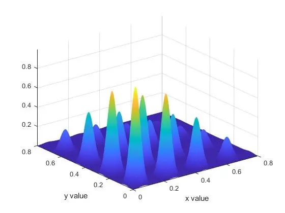
%Surface Plot
figure(1)
surfc(xx,yy,-f)
xlabel('x value')
ylabel('y value')
%Shading
shading interp
for k=1:num_cases
[inputs , fval]= ga(@stalagmite,2);
end
%Study1-Statistical Behaviour
tic
for i=1:num_cases
[inputs,fopt(i)]=ga(@stalagmite,2);
xopt(i)=inputs(1);
yopt(i)=inputs(2);
end
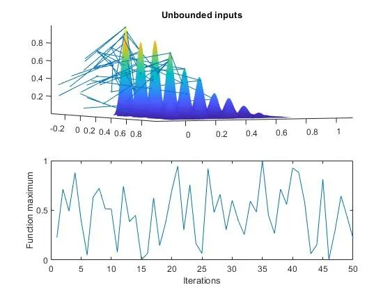
%Plotting ga with statistical behaviour
figure(2)
subplot(2,1,1)
hold on
surfc(x,y,-f)
shading interp
plot3(xopt,yopt,-fopt,'marker','.','MarkerSize',5,'MarkerFaceColor','b')
title('Unbounded inputs')
subplot(2,1,2)
plot(-fopt)
xlabel('Iterations')
ylabel('Function maximum')
study1_time=toc;
%Study2-Statistical behaviour with upper and lower bounds
tic
for i=1:num_cases
[inputs,fopt(i)]=ga(@stalagmite,2,[],[],[],[],[0:0],[0.6:0.6]);
xopt(i)=inputs(1);
yopt(i)=inputs(2);
end
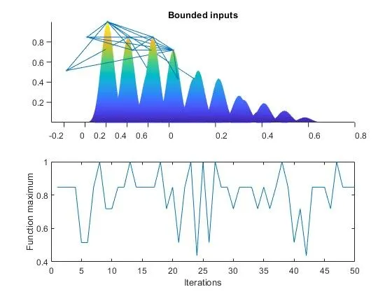
%Plotting the function with upper and lower bounds
figure(3)
subplot(2,1,1)
hold on
surfc(x,y,-f)
shading interp
plot3(xopt,yopt,-fopt,'marker','.','MarkerSize',5,'MarkerFaceColor','r')
title('Bounded inputs')
subplot(2,1,2)
plot(-fopt)
xlabel('Iterations')
ylabel('Function maximum')
study2_time=toc;
%Study3-Statistical behaviour increasing GA iterations
tic
options = optimoptions('ga');
options = optimoptions(options,'PopulationSize',300); %Defining population size
for i=1:num_cases
[inputs,fopt(i)]=ga(@stalagmite,2,[],[],[],[],[0:0],[0.6:0.6],[],[],options);
xopt(i)=inputs(1);
yopt(i)=inputs(2);
end
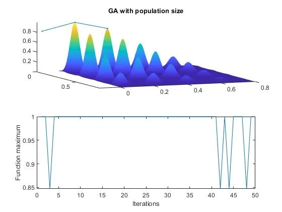
%Plotting the ga with population size
figure(4)
subplot(2,1,1)
hold on
surfc(x,y,-f)
shading interp
plot3(xopt,yopt,-fopt,'marker','.','MarkerSize',5,'MarkerFaceColor','r')
title('GA with population size')
subplot(2,1,2)
plot(-fopt)
xlabel('Iterations')
ylabel('Function maximum')
study3_time=toc;
Function Script
function f = stalagmite(input_vector)
x=input_vector(1);
y=input_vector(2);
f1_x=(sin(5.1*pi*x+0.5)).^6;
f1_y=(sin(5.1*pi*y+0.5)).^6;
f2_x=exp((-4*0.6931).*(x-0.0667)^2/(0.64));
f2_y=exp((-4*0.6931).*(y-0.0667)^2/(0.64));
f = -(f1_x.*f1_y.*f2_x.*f2_y);
end
Output plots
Stalagmite plot