Week 5 - Rayleigh Taylor Instability

RAYLEIGH-TAYLOR INSTABILITY

Aim: - To simulate the Rayleigh-Taylor instability in Ansys Fluent and state inferences based on grid-size and Atwood number.

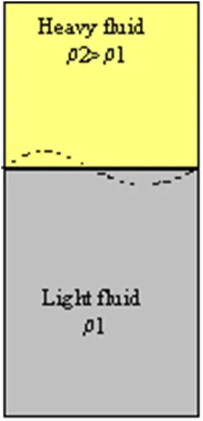
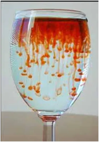
As shown, a heavier fluid rests on a lighter fluid in a container. A horizontal interface separates the two fluids. Due to gravity the situation is unstable. The surface tension stabilizes the interface whereas gravity makes it unstable. This instability is called as the Rayleigh-Taylor instability. The RT instability is buoyancy driven.

As the instability grows, the denser fluid moves down under the effect of gravitational field and the less dense fluid is displaced further upwards. This can be seen as ‘fingers’ of upper fluid inside the lower fluid.

Examples include water suspended above oil in gravity of Earth, formation of mushroom clouds from volcanoes. Water atop oil is an everyday example of Rayleigh-Taylor instability. It can be modelled as parallel layers of immiscible fluids.

PRACTICAL IMPLICATIONS

The Rayleigh-Taylor instability is an example of multiphase flow where two or more immiscible fluids interact. Multiphase flows can be modelled according to the two approaches,

• Euler-Lagrange approach
• Euler-Euler approach

We discuss the second, Euler-Euler approach

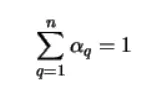
In the Euler-Euler approach, the different phases are treated mathematically as interpenetrating or mixing continuums. The concept of volume fraction is introduced to distinguish between phases. The volume fractions are assumed to be continuous functions of space and time and their sum is equal to one. The conservation equations are solved for each phase.

In ANSYS FLUENT, three different Euler-Euler multiphase models are available;

• Volume of fluid(VOF)
• Mixture model
• Eulerian model

The VOF Model

The VOF model is a surface-tracking technique applied to a fixed mesh. It is designed for two or more immiscible fluids where the position of the interface between the fluids is of interest. A single set of momentum equations is shared by the fluids and the equation of summation of volume fractions is used. Applications include stratified flows, free-surface flows, filling, sloshing, motion of large bubbles in liquid etc.

The Mixture model

Designed for two or more phases (fluids or particulates). It involves equations of momentum and prescribes relative velocities to describe the dispersed phases. Applications involve particle-laden flows sedimentation, cyclone separators etc.

The Eulerian model

The most complex model in ANSYS FLUENT. It involves a set of momentum & energy equations for each phase. Coupling is achieved using pressure & interphase exchange coeff. Examples include bubble columns, risers, fluidized beds etc.

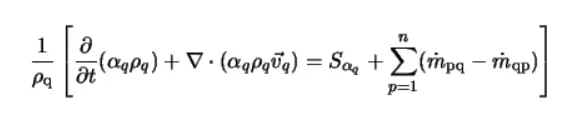
The VOF equations are as follows

Continuity

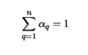
Volume fraction constraint

SIMULATION OF RT INSTABILITY IN FLUENT

1. MODELLING & SOLVING APPROACH

The Rayleigh-Taylor instability is simulated in Fluent for a 2D rectangular container. The container has primary phase air (low density fluid) in the bottom most part and secondary phase water (heavier than air) atop air.

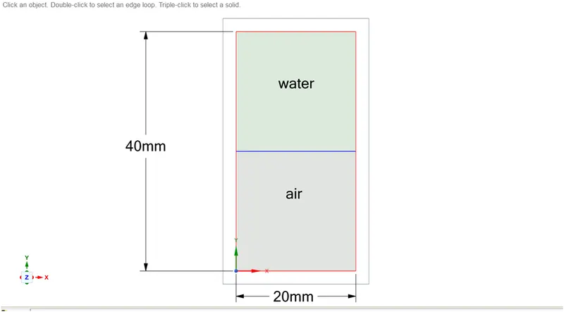
• Since density of water > density of air, the interface is unstable. The disturbances grow with time and are modelled in this simulation.
• For this case gravity forces are considered, the acceleration due to gravity is enabled in Fluent.
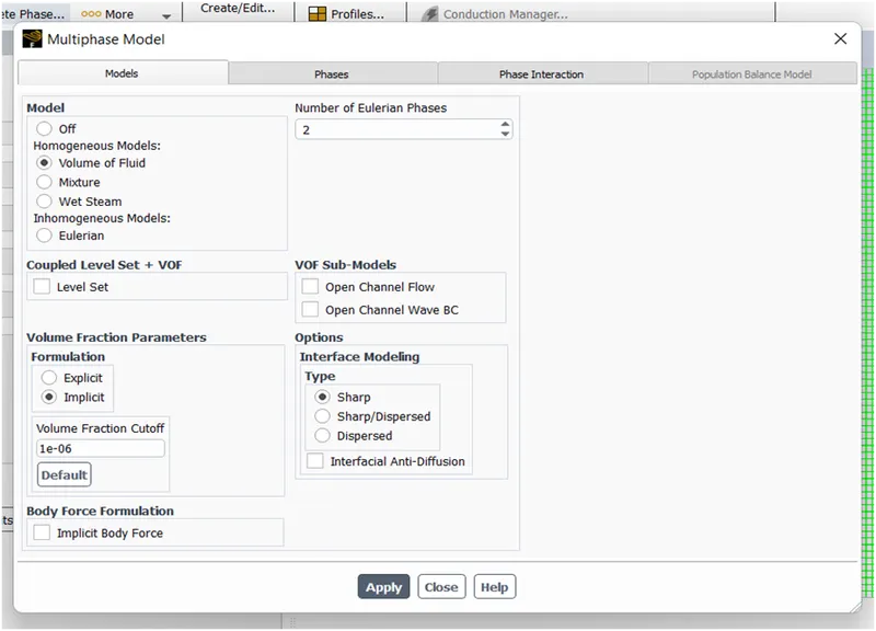
• Multiphase modelling approach is chosen, specifically the Volume of fluid (VOF) model.
• This model prescribes a volume fraction for the phases. Volume fraction is the ratio of volume of a phase to the total volume occupied by all phases.
• The momentum equation is solved for each phase which is multiplied by the volume fraction.
• The equation is constrained by;

SOLVING

• The model will be simulated for two different mesh sizes with a base mesh of 0.5 mm. Both the cases will be compared and the effect of mesh size on simulation will be discussed.
• The Rayleigh-Taylor instability is a transient process as the interface is unstable & small perturbations at the interface grow exponentially with time. A steady state simulation is of no use since it neglects the transient nature of the process.
• Another simulation with water & a user-defined material will be run for the refined mesh. The Atwood number is determined for the above two cases and the effect of variation in Atwood number on the behaviour of instability will be discussed.

2. GEOMETRY & MESH

• The geometry is a simple 2D rectangular container of size 40mm X 20mm. The length is aligned along the y-axis. The geometry is created in SpaceClaim.

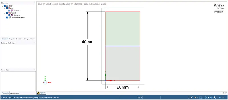
• The geometry has two components, air & water. The lowermost being air and topmost being water. The pull tool is used to create a surface.
• Share topology is enabled between the two components to facilitate the mesh creation.
• A base mesh of 5 mm is created. The number of elements being 3200.

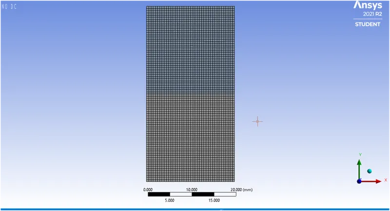
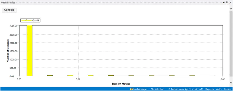
Skewness is maintained between 0-0.02 and is less than 0.8 for all the elements.

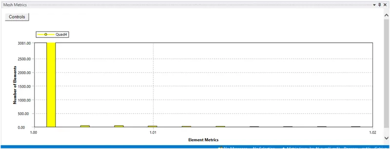
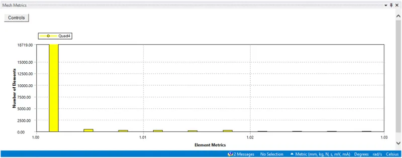
Aspect ratio is between 1-1.02 which means the elements are close to an ideal equilateral element shape.

• A refined mesh of 0.2 mm is created to observe the effect of mesh size on the simulation. The numbers of elements are 20000.

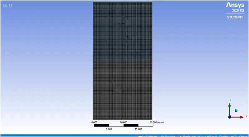
Skewness is less than 0.8.

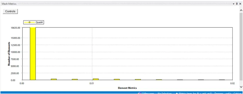
Aspect ratio between 1.0-1.03 which confirms the element shape of an equilateral element.

3. SOLVER REQUIREMENTS

• A transient state simulation based on a pressure solver is chosen.
• Multiphase model: Volume of fluid (VOF)
• Viscous: Laminar model
• Pressure-velocity coupling: SIMPLE with PRESTO for pressure & Second-order upwind schemes for momentum equations.
• A first order implicit method is chosen instead of explicit for transient formulation.
• Under relaxation factors of 0.3 for pressure & 0.7 for momentum are applied.

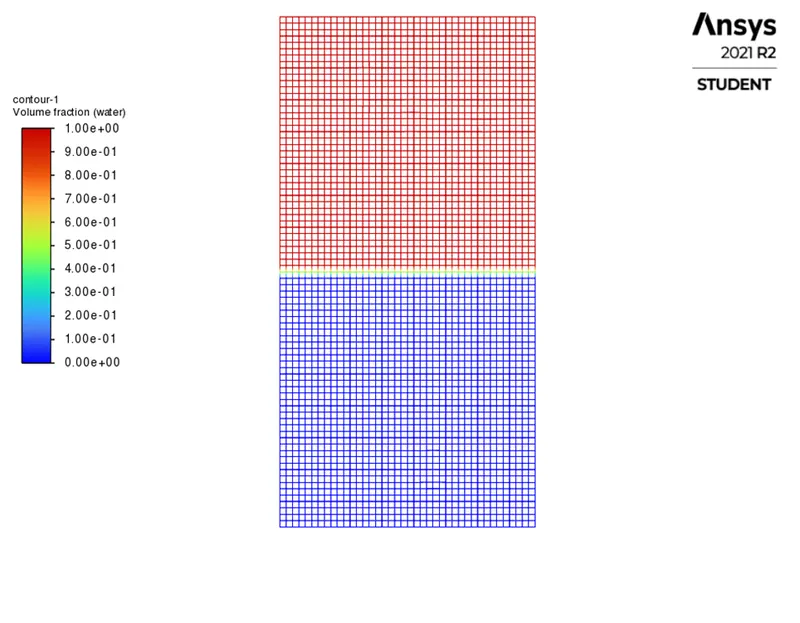
After the solution is initialized, the volume fraction is patched onto the geometry using the ‘Patch’ option in Fluent.

4. RESULTS & INFERENCES

The solution is simulated for transient state using a suitable time step size. The time step needs to be chosen suitably to avoid FPEs (floating point exception errors). This happens when the solver cannot compute an algebraic operation or mathematically speaking the solution diverges.

To avoid this, we can

• Limit the time-step.
• Apply under-relaxation.
• Mesh quality.

The under-relaxation & mesh quality parameters are already updated & checked in the solver & mesh options respectively.

Initially the time-step size increases as the flow-velocities are low and the CFL condition chooses a larger time-step. A time step of 0.005 for base mesh and 0.001 for a finer mesh is chosen.

Case A] Comparison of different mesh sizes for the same two fluids. (0.5mm & 0.2mm)

1.Initial disturbances

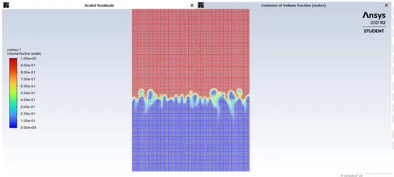
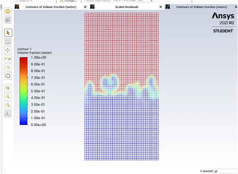
0.2 mm 0.5 mm

2. Upper fluid protruding & bubbles of lower fluid rising

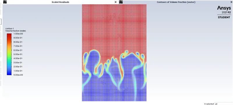
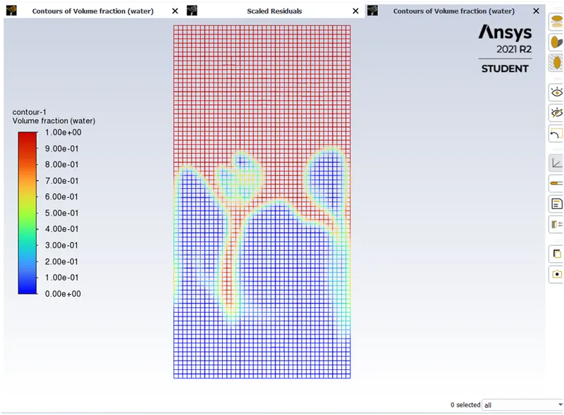
0.2 mm 0.5 mm

Google drive link for animation files : - https://drive.google.com/drive/folders/1xgU95k7lJopfbTIWYNsEi76NAwGhkjxF?usp=sharing

Inferences of comparison between mesh size

• For the mesh size of 0.5 mm, the interface captured is not as fine as compared to the 0.2 mm mesh.
• The spikes that protrude into the lighter fluid are also large for the 0.5 mm mesh and less in number, whereas for the 0.2 mm mesh, the spikes are fine and more in number.
• Large bubbles are formed in 0.5 mm as compared to 0.2mm.

Case B] Comparison between two different primary phase fluids (air & user material) and the secondary phase water for the refined mesh.

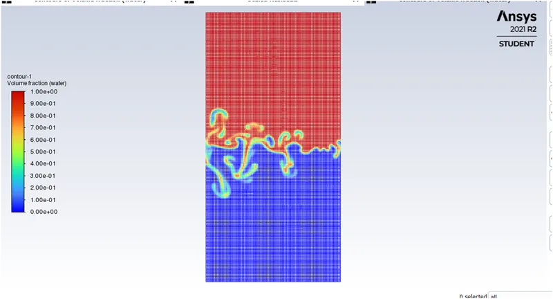
Water & air Water & user-material

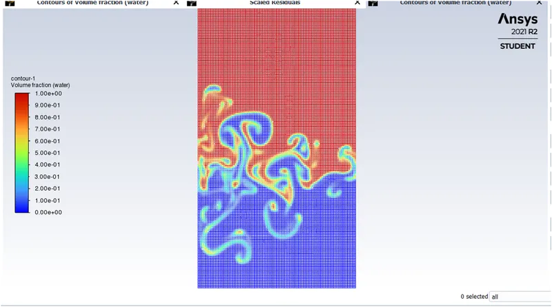
Multiple spikes of decreasing area Mushroom clouds & small spikes

Google drive link for animation files: -

https://drive.google.com/drive/folders/1xgU95k7lJopfbTIWYNsEi76NAwGhkjxF?usp=sharing

Inferences of comparison between Atwood Number for different fluids

• The Atwood number is a dimensionless number which is used in study of density stratified flows. It is a density ratio which is defined as,

At = `(rho_1-rho_2)/(rho_1+rho_2)`

where `rho_1` is the heavier fluid & `rho_2` is lighter.

• A user-defined material is used to simulate the instability between water and the material. The user-defined material has the following properties,

density = 400 kg/m^3 viscosity = 0.001 kg/(m-s)

• The material properties for air & water are,

air (density = 1.225 kg/m^3 ; viscosity = 1.7894e-05 kg/(m-s))

water(density = 998.2 kg/m^3 ; viscosity = 0.001003 kg/(m-s))

• The Atwood number for Air-water & user material-water are determined to be,
• At(air-water) = 0.9975 At(usermat-water) = 0.427835
• For large At = 0.9975 i.e. for large density differences, the bubbles that are formed are large in comparison to the spikes that protrude into the primary phase. The spikes penetrate to a larger distance in this case.
• For At = 0.428735 < 0.5 the density difference is small compared to the previous case, the spike penetrates to a lesser extent. The size of the spikes decreases as it penetrates further. The difference in sizes of the spikes & bubbles are small. Mushroom shaped clouds of lighter fluid are formed inside the heavier fluid.