Week 5.1 - Mid term project - Solving the steady and unsteady 2D heat conduction problem
UNSTEADY STATE ANALYSIS
The unsteady 2d heat conduction equation is given by
`(delT)/(delt) = kappa*((del^2T)/(delx^2) + (del^2T)/(dely^2) )`
It is a parabolic PDE, which lend themselves to marching solutions.
By using forward-difference scheme for the time derivative and central-differencing scheme for spatial derivatives, the equation can be discretized.
`(T_(i,j)^(n+1)−T_(i,j)^(n))/(Δt)` = `D[(T_(i+1,j)−2T_(i,j)+T_(i−1,j))/(2*Δx)+(T_(i,j+1)−2T_(i,j)+T_(i,j−1))/(2*Δy)]^(n,n+1)`
where index 'n' refers to time step & 'i,j' refers to grid points.
for explicit scheme 'n', for implicit 'n+1'
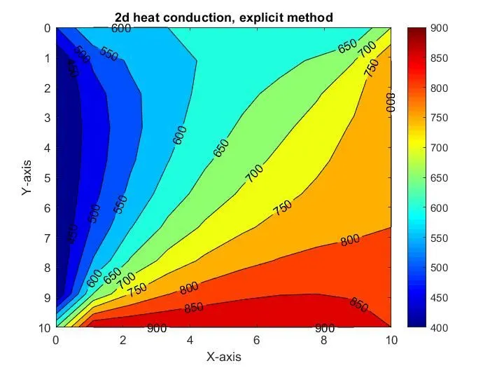
A] For transient state, the explicit scheme code is,
number of iterations for this method are 500.
clear all
close all
clc

%Specifying the domain which is a unit length square plate
nx = 10; %grid points in x
ny = 10; %grid points in y
x = 1:nx;
y = 1:ny;
dx = abs(x(2)-x(1));
dy = abs(y(2)-y(1));
%Time step
alpha = 1.2;
dt = 0.1;

%Boundary conditions
T_top = 600;
T_bottom = 900;
T_left = 400;
T_right = 800;

%Create a temperature array
T = 300*ones(ny,nx);

%assign arrays
%top  column = 2 : 9,  row = 1
t_r = 1;
t_cs = 2;
t_ce = 9;
T(t_r, t_cs:t_ce) = 600;

%bottom  column = 2 : 9, row = 10
b_r = 10;
b_cs = 2;
b_ce = 9;
T(b_r, b_cs : b_ce) = 900;

%left  column = 1, row = 2:9
l_c = 1;
l_rs = 2;
l_re = 9;
T(l_rs : l_re, l_c) = 400;

%right column = 10, row = 2:50
r_c = 10;
r_rs = 2;
r_re = 9;
T(r_rs:r_re, r_c) = 800;

T(1,1) = 500;
T(10,1) = 650;
T(1,10) = 700;
T(10,10) = 850;

%specify previous values for marching solution
Told = T;

%simplifying the equation
k1 = alpha*(dt/(dx)^2);
k2 = alpha*(dt/(dy)^2);

cfl = alpha*((1/dx^2) + (1/dy^2))*dt ;

%initialize error terms
error_mag = 1;
error_req = 1e-4;

iterations = 0;
%time loop, marching solution
for nt = 1 : 500

    %spatial loop
   for i = 2 : nx-1
      for j = 2 : ny-1
        H = (Told(i-1,j) -2*Told(i,j)+ Told(i+1,j));
        V = (Told(i,j-1) -2*Told(i,j)+ Told(i,j+1));
        T(i,j) = Told(i,j) + (H*k1) + (V*k2);

     end
  end
 iterations = iterations+1;

 Told = T;

x = linspace(0,10,nx);
y = linspace(0,10,ny);
[X,Y] = meshgrid(x,y);
[c,h] = contourf(X,Y,T);
clabel(c,h)
colorbar
colormap(jet)
set(gca,'Ydir','reverse')
pause(0.01)
xlabel('X-axis');
ylabel('Y-axis');
title({['2d heat conduction, explicit method'],['CFL =',num2str(cfl)]})
end
For explicit method, the number of iterations required are equal to the number of time steps. Thus, if a problem requires much time to reach steady state, i.e. more number of time steps, the number of iterations would also increase.
IMPLICIT METHOD
For implicit methods, we we compute values at a timestep, using values at that timestep and previous timestep values.
To implement this , we use iterative solvers, which using a initial guess, compute values in an iterative manner
B] Jacobi
The Jacobi method computes 'k+1'th approximation using 'k'th value.
For Ax = b
L : lower triangular matrix of A
U : Upper triangular matrix of A
`x^(m+1) = b - L*x^(m) - U*x^(m)`
The number of iterations are 155.
clear all
close all
clc

nx = 10; %grid points in x
ny = 10; %grid points in y
x = 1:nx;
y = 1:ny;
dx = abs(x(2)-x(1));
dy = abs(y(2)-y(1));
c = 1.2;
dt = 10;

%Boundary conditions
T_top = 600;
T_bottom = 900;
T_left = 400;
T_right = 800;

T = 300*ones(nx,ny);

%assign arrays
%top  column = 2 : 9,  row = 1
t_r = 1;
t_cs = 2;
t_ce = 9;
T(t_r, t_cs:t_ce) = 600;

%bottom  column = 2 : 9, row = 10
b_r = 10;
b_cs = 2;
b_ce = 9;
T(b_r, b_cs : b_ce) = 900;

%left  column = 1, row = 2:9
l_c = 1;
l_rs = 2;
l_re = 9;
T(l_rs : l_re, l_c) = 400;

%right column = 10, row = 2:50
r_c = 10;
r_rs = 2;
r_re = 9;
T(r_rs:r_re, r_c) = 800;

T(1,1) = 500;
T(10,1) = 650;
T(1,10) = 700;
T(10,10) = 850;

Tinitial = T;
Told = T;

k1 = c*(dt/(dx)^2);
k2 = c*(dt/(dy)^2);
term1 = 1*((1 + (2*k1) + (2*k2))^-1);
term2 = k1*term1;
term3 = k2*term1;
error_mag = 1;
error_req = 1e-4;

iteration = 0;

for nt = 1500

    while error_mag > error_req

        for j = 2:(ny-1)

            for i = 2:(nx-1)

                term1 = 1*((1 + (2*k1) + (2*k2))^-1);
                term2 = k1*term1;
                term3 = k2*term1;
                H = (Told(i-1,j) + Told(i+1,j));
                V = (Told(i,j-1) + Told(i,j+1));
                T(i,j) = (Tinitial(i,j)*term1) + (H*term2) + (V*term3);

            end
        end
        %calculating error to determine convergence
        error_mag = max(max(abs(Told - T)));
        %updating 'Told' to 'T' for further iterations
        Told = T;
        iteration = iteration+1;
    end

    %Updating previous timestep values to new values
    Tinitial = T;

end

figure(1)
[X,Y] = meshgrid(x,y);
[c,h] = contourf(X,Y,T)
clabel(c,h)
set(gca,'Ydir','reverse')
colorbar
colormap(jet)
pause(0.01)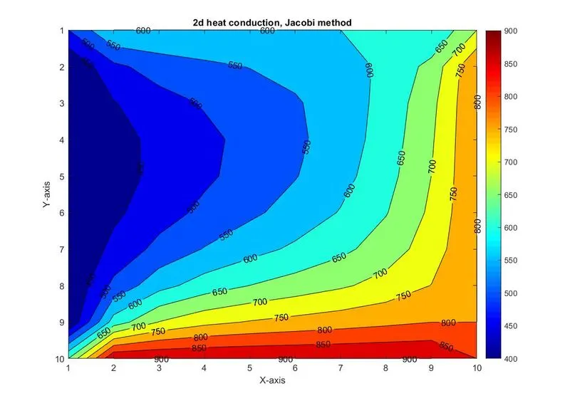
C] Gauss Seidel
The Gauss Seidel method is a method of succesive corrections, which replaces old approximations by new approximations as soon as the later are calculated.
For Ax = b
`x^(m+1) = b - L*x^(m+1) - U*x^(m)`
where L: Lower triangular matrix of 'A'
U : Upper triangular matrix of 'A'
The number of iterations are 84.
clear all
close all
clc

nx = 10; %grid points in x
ny = 10; %grid points in y
x = 1:nx;
y = 1:ny;
dx = abs(x(2)-x(1));
dy = abs(y(2)-y(1));
c = 1.2;
dt = 10;

%Boundary conditions
T_top = 600;
T_bottom = 900;
T_left = 400;
T_right = 800;

T = 300*ones(nx,ny);

%assign arrays
%top  column = 2 : 9,  row = 1
t_r = 1;
t_cs = 2;
t_ce = 9;
T(t_r, t_cs:t_ce) = 600;

%bottom  column = 2 : 9, row = 10
b_r = 10;
b_cs = 2;
b_ce = 9;
T(b_r, b_cs : b_ce) = 900;

%left  column = 1, row = 2:9
l_c = 1;
l_rs = 2;
l_re = 9;
T(l_rs : l_re, l_c) = 400;

%right column = 10, row = 2:50
r_c = 10;
r_rs = 2;
r_re = 9;
T(r_rs:r_re, r_c) = 800;

T(1,1) = 500;
T(10,1) = 650;
T(1,10) = 700;
T(10,10) = 850;

Tinitial = T;
Told = T;

k1 = c*(dt/(dx)^2);
k2 = c*(dt/(dy)^2);
term1 = 1*((1 + (2*k1) + (2*k2))^-1);
term2 = k1*term1;
term3 = k2*term1;
error_mag = 1;
error_req = 1e-4;

iteration = 0;

for nt = 1500

    while error_mag > error_req

        for j = 2:(ny-1)

            for i = 2:(nx-1)

                term1 = 1*((1 + (2*k1) + (2*k2))^-1);
                term2 = k1*term1;
                term3 = k2*term1;
                H = (T((i-1),j) + Told((i+1),j));
                V = (T(i,(j-1)) + Told(i,(j+1)));
                T(i,j) = (Tinitial(i,j)*term1) + (H*term2) + (V*term3);

            end
        end

        error_mag = max(max(abs(Told - T)));

        Told = T;
        iteration = iteration+1;
    end

    Tinitial = T;
end

figure(1)
[X,Y] = meshgrid(x,y);
[c,h] = contourf(X,Y,T);
clabel(c,h)
set(gca,'Ydir','reverse')
colorbar
colormap(jet)
pause(0.01)
xlabel('X-axis');
ylabel('Y-axis');
title('2d heat conduction, Gauss-Seidel method') 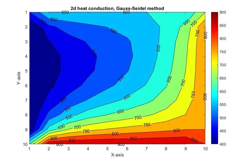
D] Successive over relaxation
The SOR method is a variant of the Gauss Seidel method which is used for fast convergence.
`x^(m+1) = (1-omega)*x^(m) + omega*(x(GS))`
where `omega` is the relaxation factor. It enhances the values calculated by Gauss-Seidel. It is usually greater than 1.
The number of iterations are 56.
clear all
close all
clc

nx = 10; %grid points in x
ny = 10; %grid points in y
x = 1:nx;
y = 1:ny;
dx = abs(x(2)-x(1));
dy = abs(y(2)-y(1));
c = 1.2;
dt = 10;

%Boundary conditions
T_top = 600;
T_bottom = 900;
T_left = 400;
T_right = 800;

T = 300*ones(nx,ny);

%assign arrays
%top  column = 2 : 9,  row = 1
t_r = 1;
t_cs = 2;
t_ce = 9;
T(t_r, t_cs:t_ce) = 600;

%bottom  column = 2 : 9, row = 10
b_r = 10;
b_cs = 2;
b_ce = 9;
T(b_r, b_cs : b_ce) = 900;

%left  column = 1, row = 2:9
l_c = 1;
l_rs = 2;
l_re = 9;
T(l_rs : l_re, l_c) = 400;

%right column = 10, row = 2:50
r_c = 10;
r_rs = 2;
r_re = 9;
T(r_rs:r_re, r_c) = 800;

T(1,1) = 500;
T(10,1) = 650;
T(1,10) = 700;
T(10,10) = 850;

Tinitial = T;
Told = T;

k1 = c*(dt/(dx)^2);
k2 = c*(dt/(dy)^2);
term1 = 1*((1 + (2*k1) + (2*k2))^-1);
term2 = k1*term1;
term3 = k2*term1;
error_mag = 1;
error_req = 1e-4;

iteration = 0;
%relaxation factor
alpha = 1.2;

for nt = 1500

    while error_mag > error_req

        for j = 2:(ny-1)

            for i = 2:(nx-1)

                term1 = 1*((1 + (2*k1) + (2*k2))^-1);
                term2 = k1*term1;
                term3 = k2*term1;
                H = (T((i-1),j) + Told((i+1),j));
                V = (T(i,(j-1)) + Told(i,(j+1)));
                %Calculating the Gauss Seidel term
                T(i,j) = (Tinitial(i,j)*term1) + (H*term2) + (V*term3);
                %SOR method using Gauss Seidel term
                T(i,j) = ((1-alpha)*Told(i,j)) + alpha*T(i,j);
            end
        end

        error_mag = max(max(abs(Told - T)));

        Told = T;
        iteration = iteration+1;
    end

    Tinitial = T;
end

figure(1)
[X,Y] = meshgrid(x,y);
[c,h] = contourf(X,Y,T);
clabel(c,h)
set(gca,'Ydir','reverse')
colorbar
colormap(jet)
pause(0.01)
xlabel('X-axis');
ylabel('Y-axis');
title('2d heat conduction, Successive over relaxation method')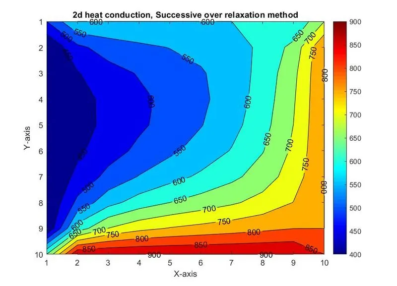
The order of 'iterations required for convergence' is
Jacobi > Gauss Seidel > SOR
STEADY STATE ANALYSIS
The equation of 2d heat conduction for a steady state is
`(del^2T)/(delx^2) + (del^2T)/(dely^2) = 0`
also called as the Laplacian equation
The discretized equation is
`T_(i,j) = (dx^2*dy^2)/(2*(dx^2 + dy^2)) * [(T_(i-1,j) + T_(i+1,j))/(dx^2) + (T_(i,j-1) + T_(i,j+1))/(dy^2)]`
Using iterative solver,
A] For Jacobi, the equation is
`T_(i,j) = (dx^2*dy^2)/(2*(dx^2 + dy^2)) * [(T_(old*(i-1,j) )+ T_(old(i+1,j)))/(dx^2) + (T_(old(i,j-1)) + T_(old(i,j+1)))/(dy^2)]`
The number of iterations are 207.
clear all
close all
clc


nx = 10; %grid points in x
ny = 10; %grid points in y
x = 1:nx;
y = 1:ny;
dx = abs(x(2)-x(1));
dy = abs(y(2)-y(1));

%Boundary conditions
T_top = 600;
T_bottom = 900;
T_left = 400;
T_right = 800;

T = 300*ones(nx,ny);

%assign arrays
%top  column = 2 : 9,  row = 1
t_r = 1;
t_cs = 2;
t_ce = 9;
T(t_r, t_cs:t_ce) = 600;

%bottom  column = 2 : 9, row = 10
b_r = 10;
b_cs = 2;
b_ce = 9;
T(b_r, b_cs : b_ce) = 900;

%left  column = 1, row = 2:9
l_c = 1;
l_rs = 2;
l_re = 9;
T(l_rs : l_re, l_c) = 400;

%right column = 10, row = 2:50
r_c = 10;
r_rs = 2;
r_re = 9;
T(r_rs:r_re, r_c) = 800;

T(1,1) = 500;
T(10,1) = 650;
T(1,10) = 700;
T(10,10) = 850;
Told = T;
%simplifying the equation
k = (dx^2 * dy^2)/(2*(dx^2 + dy^2));

error_mag = 1;
error_req = 1e-4;
iteration = 0;


    while error_mag > error_req

        for j = 2:(ny-1)

            for i = 2:(nx-1)

                %
                H = (Told(i-1,j) + Told(i+1,j))/(dx^2);
                V = (Told(i,j-1) + Told(i,j+1))/(dy^2);
                T(i,j) = k*( H + V);

            end
        end

        error_mag = max(max(abs(Told - T)));

        Told = T;
        iteration = iteration+1;
    end


figure(1)
[X,Y] = meshgrid(x,y);
[c,h] = contourf(X,Y,T);
clabel(c,h)
set(gca,'Ydir','reverse')
colorbar
colormap(jet)
pause(0.01)
xlabel('X-axis');
ylabel('Y-axis');
title('Steady state, Jacobi method')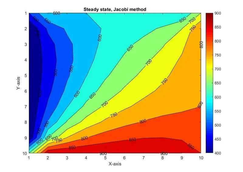
B] Gauss Seidel
`T_(i,j) = (dx^2*dy^2)/(2*(dx^2 + dy^2)) * [(T_(i-1,j) + T_(old(i+1,j)))/(dx^2) + (T_(i,j-1) + T_(old(i,j+1)))/(dy^2)]`
The number of iterations are 111.
clear all
close all
clc


nx = 10; %grid points in x
ny = 10; %grid points in y
x = 1:nx;
y = 1:ny;
dx = abs(x(2)-x(1));
dy = abs(y(2)-y(1));

%Boundary conditions
T_top = 600;
T_bottom = 900;
T_left = 400;
T_right = 800;

T = 300*ones(nx,ny);

%assign arrays
%top  column = 2 : 9,  row = 1
t_r = 1;
t_cs = 2;
t_ce = 9;
T(t_r, t_cs:t_ce) = 600;

%bottom  column = 2 : 9, row = 10
b_r = 10;
b_cs = 2;
b_ce = 9;
T(b_r, b_cs : b_ce) = 900;

%left  column = 1, row = 2:9
l_c = 1;
l_rs = 2;
l_re = 9;
T(l_rs : l_re, l_c) = 400;

%right column = 10, row = 2:50
r_c = 10;
r_rs = 2;
r_re = 9;
T(r_rs:r_re, r_c) = 800;

T(1,1) = 500;
T(10,1) = 650;
T(1,10) = 700;
T(10,10) = 850;
Told = T;
k = (dx^2 * dy^2)/(2*(dx^2 + dy^2));

error_mag = 1;
error_req = 1e-4;
iteration = 0;


    while error_mag > error_req

        for j = 2:(ny-1)

            for i = 2:(nx-1)


                H = (T(i-1,j) + Told(i+1,j))/(dx^2);
                V = (T(i,j-1) + Told(i,j+1))/(dy^2);
                T(i,j) = k*( H + V);

            end
        end

        error_mag = max(max(abs(Told - T)));

        Told = T;
        iteration = iteration+1;
    end


figure(1)
[X,Y] = meshgrid(x,y);
[c,h] = contourf(X,Y,T);
clabel(c,h)
set(gca,'Ydir','reverse')
colorbar
colormap(jet)
pause(0.01)
xlabel('X-axis');
ylabel('Y-axis');
title('Steady state, Gauss-Seidel method')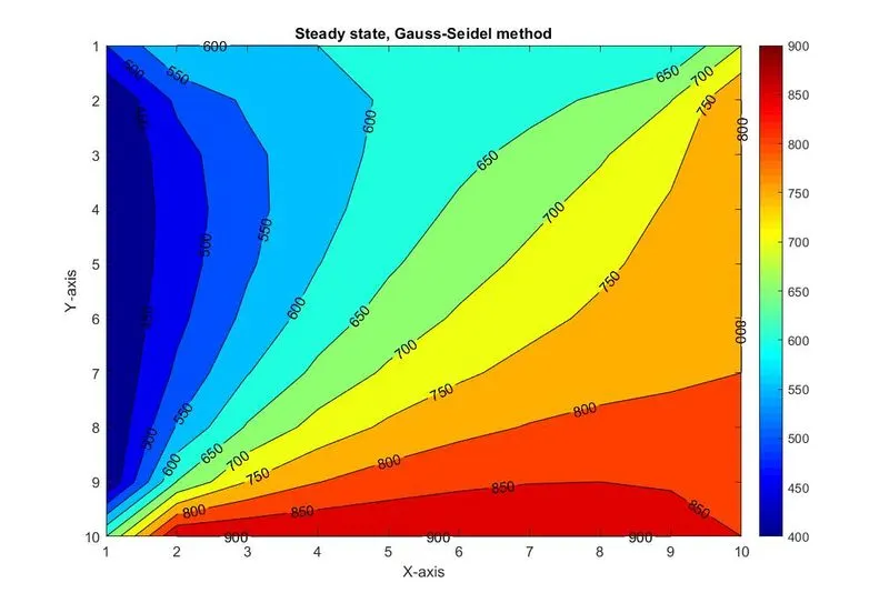
C] Successive over relaxation
`T_(i,j) = (1-omega)*T_(old(i,j)) + (omega*T_(GS))`
`omega` is the relaxation factor
`T_(GS)` is obtained from Gauss Seidel method.
The number of iterations are 75.
clear all
close all
clc


nx = 10; %grid points in x
ny = 10; %grid points in y
x = 1:nx;
y = 1:ny;
dx = abs(x(2)-x(1));
dy = abs(y(2)-y(1));

%Boundary conditions
T_top = 600;
T_bottom = 900;
T_left = 400;
T_right = 800;

T = 300*ones(nx,ny);

%assign arrays
%top  column = 2 : 9,  row = 1
t_r = 1;
t_cs = 2;
t_ce = 9;
T(t_r, t_cs:t_ce) = 600;

%bottom  column = 2 : 9, row = 10
b_r = 10;
b_cs = 2;
b_ce = 9;
T(b_r, b_cs : b_ce) = 900;

%left  column = 1, row = 2:9
l_c = 1;
l_rs = 2;
l_re = 9;
T(l_rs : l_re, l_c) = 400;

%right column = 10, row = 2:50
r_c = 10;
r_rs = 2;
r_re = 9;
T(r_rs:r_re, r_c) = 800;

T(1,1) = 500;
T(10,1) = 650;
T(1,10) = 700;
T(10,10) = 850;
Told = T;
k = (dx^2 * dy^2)/(2*(dx^2 + dy^2));

error_mag = 1;
error_req = 1e-4;
iteration = 0;

%relaxation factor
omega = 1.2;


    while error_mag > error_req

        for j = 2:(ny-1)

            for i = 2:(nx-1)


                H = (T(i-1,j) + Told(i+1,j))/(dx^2);
                V = (T(i,j-1) + Told(i,j+1))/(dy^2);
                T(i,j) = k*( H + V);
                T(i,j) = ((1-omega)*Told(i,j)) + (omega*T(i,j));
            end
        end

        error_mag = max(max(abs(Told - T)));

        Told = T;
        iteration = iteration+1;
    end


figure(1)
[X,Y] = meshgrid(x,y);
[c,h] = contourf(X,Y,T);
clabel(c,h)
set(gca,'Ydir','reverse')
colorbar
colormap(jet)
pause(0.01)
xlabel('X-axis');
ylabel('Y-axis');
title('Steady state, SOR method')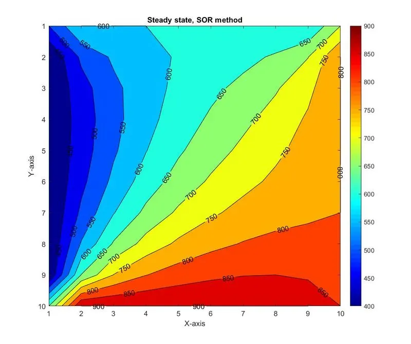
For steady state the SOR method approaches convergence using the least iterations followed by Gauss Seidel then Jacobi.