Week 1- Mixing Tee
INTRODUCTION
The 'Tee' geometry or mixing Tee, is commonly employed where two fluid streams with different physical properties mix together, for example petroleum industry, HVAC systems. The effectiveness of mixing T can be defined in terms of uniformity of the properties at the outlet, for example temperature. The fluid properties at both the inlets are usually different. Temperature differences lead to heat transfer and the final mixture attains a steady uniform temperature. The velocity at either of the inlets affects the mixing process and the mixture temperature is affected if either of the velocity is increased or decreased.
The length of the pipe is also a factor to consider. Pipe length affects the development of flow pattern. The flow usually becomes turbulent in longer pipes which helps in effective mixing of fluids.
OBJECTIVES
For this study, a comparison of two cases, a short Tee and a long Tee is done. They are compared based on
1)Cell count
2)Average outlet temperature
3)Iterations required for convergence.
4)The effect of length of the Tee and momentum ratio(velocity at cold inlet/velocity at hot inlet) is also discussed.
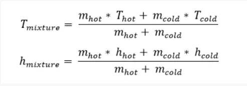
The standard deviation is a measure of how close the actual value is to the mean value. A high standard deviation indicates that the values are spread over a wider range. The standard deviation of temperature at the outlet is calculated in Ansys and plotted along number of iterations. The results are then compared with the theoretical values of temperature which are calculated using,
GEOMETRY & MESH
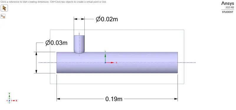
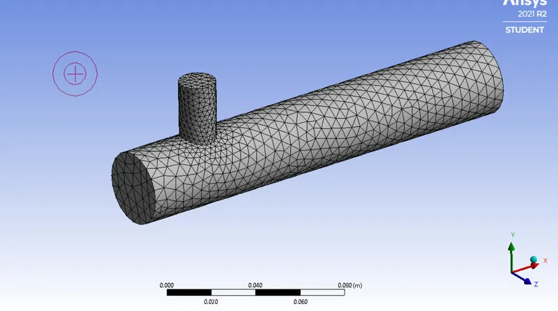
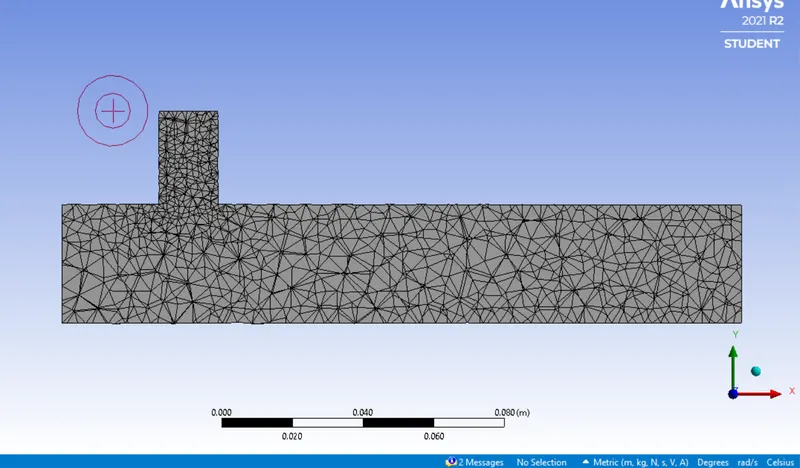
The geometry is a pipe with circular cross sectional area, it consists of a main pipe and a smaller second inlet. After a short distance along the length of main pipe there is a junction at which another pipe of smaller diameter acts as a second inlet. The geometry is imported in SpaceClaim and cleaned up using volume extraction feature which hides those surfaces which are of less importance for the flow simulation and suppress the physics for those surfaces.
The coordinate directions are aligned as shown. 'X' along the main pipe and 'Y' along the smaller second inlet.
The dimensions of the geometry are, D = 0.032m d = 0.02m length = 0.19m .
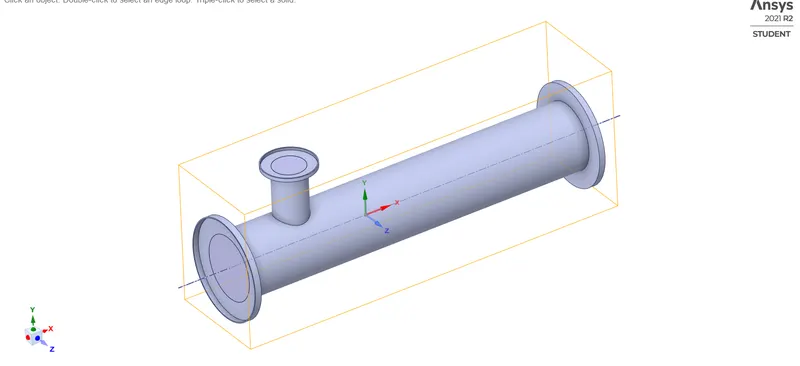
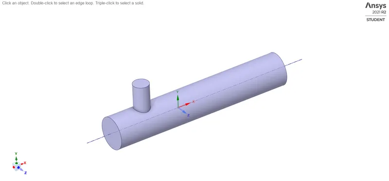
The geometry of short mixing T before and after fluid volume extraction.
---
The mesh element is of tetrahedral shape. Default size of mesh is used which is of size 0.01 m.
The mesh metrics histogram is,
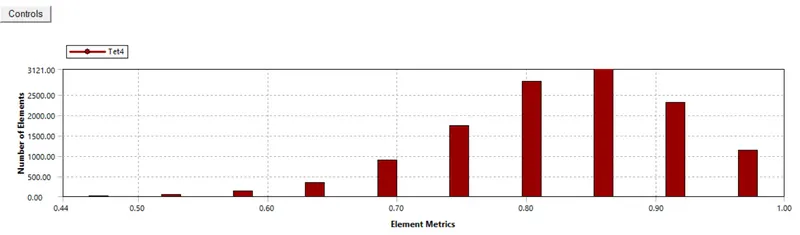
As seen from the histogram, most of the elements are above 50% which indicates a good quality mesh.
BOUNDARY CONDITIONS AND SOLUTION INITIALIZATION
The solver is selected to be of steady state, which solves the fluid continuity, momentum as well as the energy equation.
The boundary conditions are,
inlet x:- velocity = 3 m/s, temperature = 36° C
inlet y:- velocity = based on momentum ratio, temperature = 19° C
pipe wall:- no slip
outlet:- pressure based, P = 0 Pa (gauge pressure).
Solution initialization is done to provide the solver with an initial 'guess' of the flow field properties, provided in the interior of the flow domain using various methods.
Solution initialization in Ansys Fluent is done using the Hybrid initialization. Hybrid initialization is a collection of interpolation methods which solves the Laplace equation to determine the velocity and pressure fields.
The flow is simulated in Ansys Fluent. The models selected to simulate turbulence are k-epsilon and k-omega.
These models are based on the RANS (Reynolds Averaged Navier Stokes) equations for turbulence. In these equations the fluid velocity is assumed to have two parts, a mean velocity and a fluctuating velocity.
u = `overline u + dotu`
k-epsilon and k-omega solve for the kinetic energy(k) and dissipation rate(epsilon,omega) of turbulence.
Case1 Short T
Using k-epsilon
A] Momentum ratio = 2
Hot Inlet x velocity = 3 m/s temperature = 36° C
Cold Inlet y velocity = 6 m/s temperature = 19° C
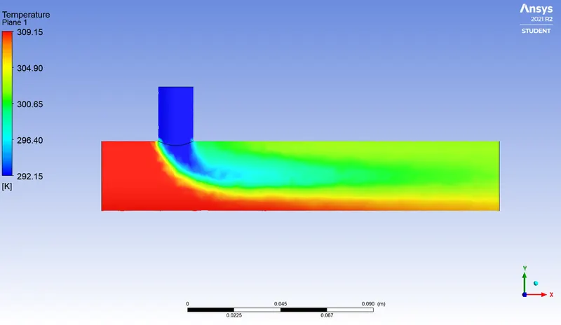
Contours
1) Along the length
Temperature contour Velocity contour
2) Across the cross section
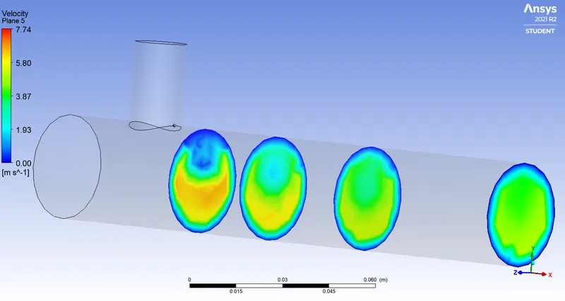
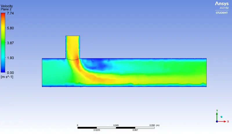
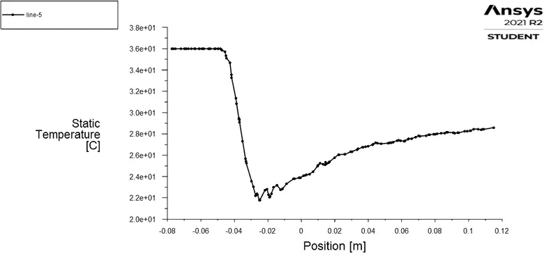
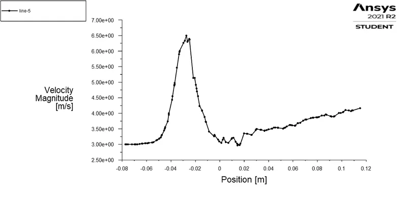
The cold stream does not reach the opposite wall of the pipe and changes its direction not far from the corner. At the outlet both the temperature and the velocity profile are not uniform and have different values along the cross section indicating that the streams have not mixed quite properly.
Line plots
Temperature Velocity
Residuals
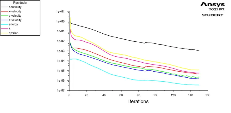
Results
| Momentum Ratio | Cell count | Average outlet Temperature | Iterations required | Standard deviation of temperature | |
| Result | Theoretical | ||||
|
2 |
30.25 | 30.324 | 50 |
1.7 |
|
B] Momentum ratio = 4
Hot Inlet x velocity = 3 m/s temperature = 36° C
Cold Inlet y velocity = 12 m/s temperature = 19° C
Temperature contour Velocity contour
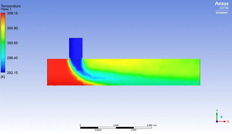
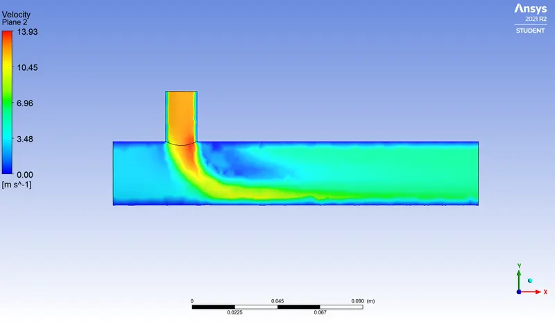
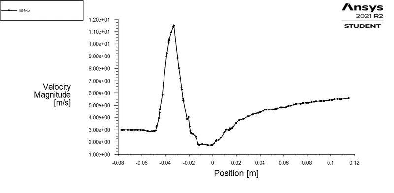
The cold stream reaches the opposite wall after getting deflected and the temperature and velocity are more uniform as compared to previous.
Line plots
Temperature Velocity
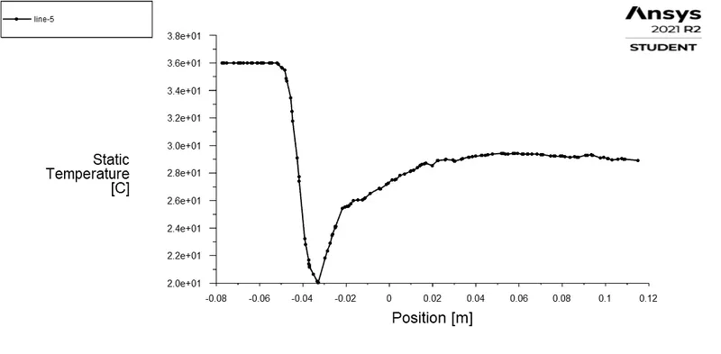
Residuals
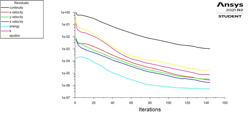
Results
| Momentum Ratio | Cell count | Average outlet Temperature | Iterations required | Standard deviation of temperature | |
| Result | Theoretical | ||||
|
4 |
27.5 | 27.4876 | 70 |
0.88 |
|
Comparsion of results for A] & B] for k-epsilon model,
| Momentum Ratio | Cell count | Average outlet Temperature | Iterations required | Standard deviation of temperature | |
| Result | Theoretical | ||||
|
2 |
30.25 | 30.324 | 50 |
1.7 |
|
|
4 |
27.5 | 27.4876 | 70 |
0.88 |
|
The standard deviation for momentum ratio 2 is more than that for momentum ratio of 4. A higher momentum ratio also requires more number of iterations in turn more time for convergence.
Using k-omega SST,
A] Momentum ratio = 2
Temperature contour Velocity contour
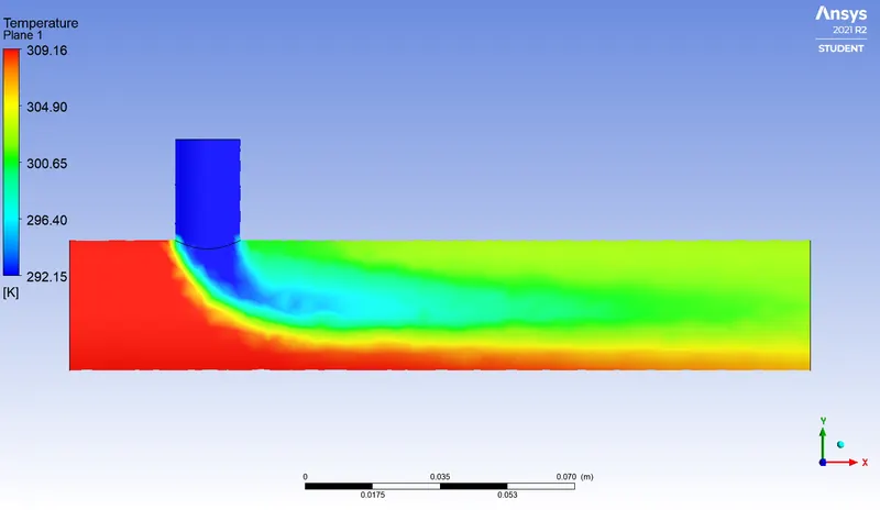
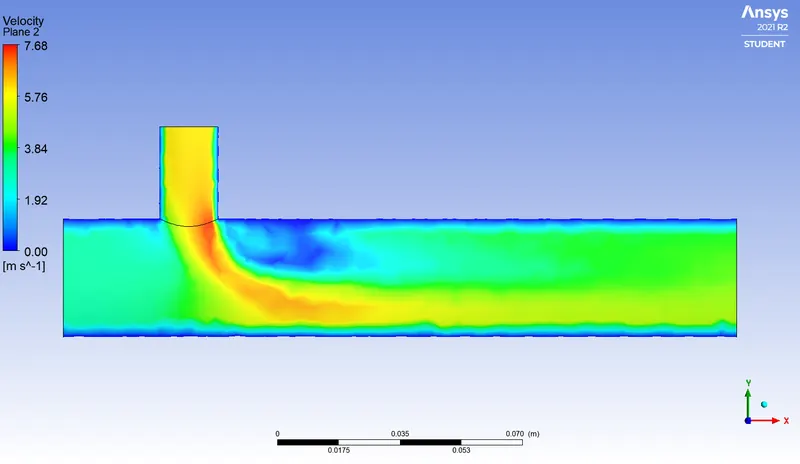
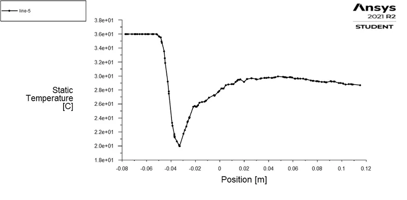
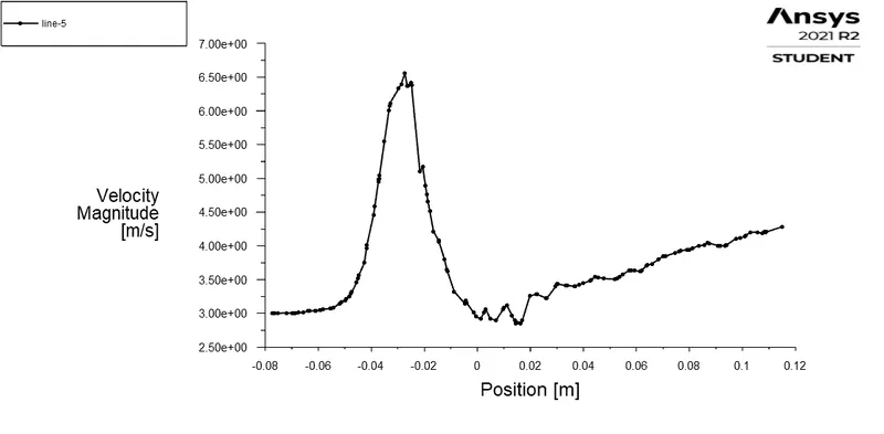
Line plots
Temperature Velocity
B] Momentum ratio = 4
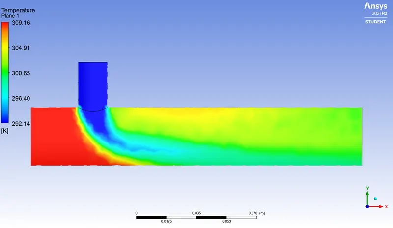
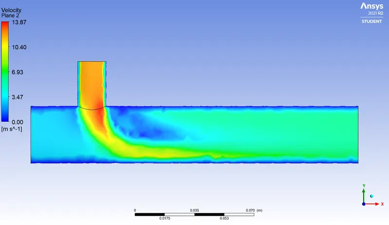
Temperature contour Velocity contour
Line plots
Temperature Velocity
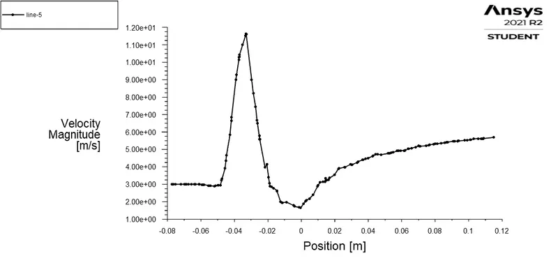
By running both of the above parts using the k-omega SST model, the results are as follows.
| Momentum Ratio | Cell count | Average outlet Temperature | Iterations required | Standard deviation of temperature | |
| Result | Theoretical | ||||
|
2 |
30.25 | 30.324 | 60 |
1.5 |
|
|
4 |
27.5 | 27.4876 | 80 |
0.7750 |
|
Though k-omega SST takes more number of iterations to achieve convergence, the standard deviation is lesser than k-epsilon. Thus it implies more uniform conditions at the outlet.
Therefore, k-omega SST is most suitable for this case and for simulating a similar flow in a long T, we shall use this model.
Case2 Long T
k-omega SST
A] Momentum ratio = 2
Hot Inlet x velocity = 3 m/s temperature = 36° C
Cold Inlet y velocity = 6 m/s temperature = 19° C
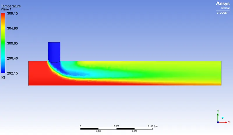
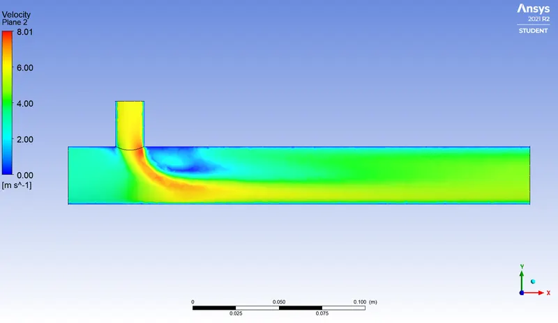
Temperature contour Velocity contour
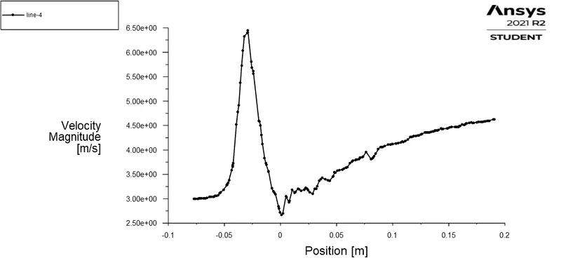
Line plots
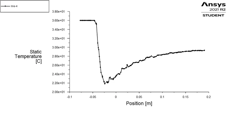
Temperature Velocity
Residuals
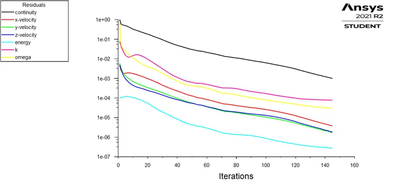
| Momentum Ratio | Cell count | Average outlet Temperature | Iterations required | Standard deviation of temperature | |
| Result | Theoretical | ||||
|
2 |
17768 | 30.3 | 30.324 | 65 |
0.9 |
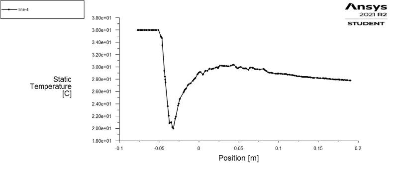
By using a long T, the temperature is closer to the actual value and the standard deviation has also decreased.
B] Momentum ratio = 4
Hot Inlet x velocity = 3 m/s temperature = 36° C
Cold Inlet y velocity = 12 m/s temperature = 19° C
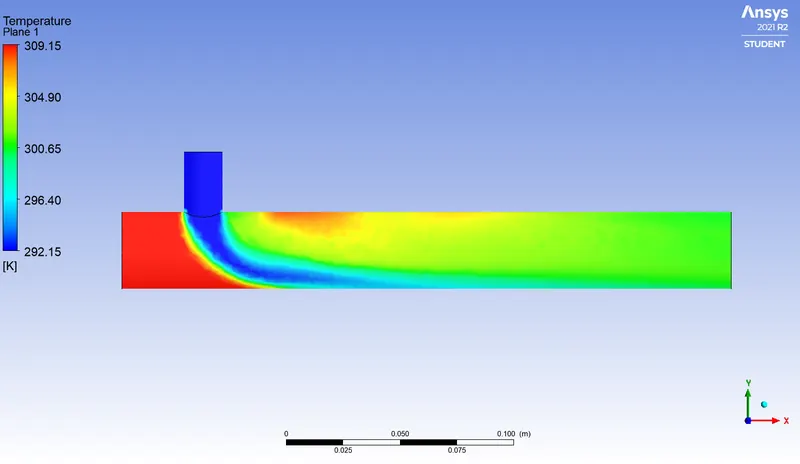
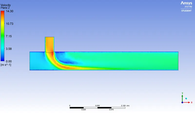
Temperature contour Velocity contour
Line plots
Temperature Velocity
Residual
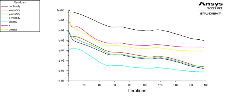
The results further improve after the momentum ratio is increased. The standard deviation decreases to 0.4.
| Momentum Ratio | Cell count | Average outlet Temperature | Iterations required | Standard deviation of temperature | |
| Result | Theoretical | ||||
|
4 |
17768 | 27.4 | 27.4876 | 65 |
0.42 |
Thus it is concluded that a long mixing T with a higher momentum ratio gives better results as compared to a short mixing T.
The k-omega SST model is a suitable choice for simulating such type of flows.
GRID INDEPENDENCE TEST
For the long mixing T, the flow is simulated for smaller mesh sizes of 0.002 m and 0.003 m & the results are as follows,
| Mesh size in mm | cell count | Iterations required | Standard deviation |
| 5 | 17768 | 65 | 0.4 |
| 3 | 56273 | 80 | 0.6 |
| 2 | 139096 | 100 | 0.9 |
Smaller mesh sizes requires more number of iterations and there is a slight increase in the standard deviation.
Hence a mesh size of 0.005 is the most suitable.