Week 9 - FVM Literature Review
1] The FVM is a numerical method for evaluating partial differential equations. Finite volume method uses the integral form of the conservation law. The domain is divided into many control volumes and the conservation laws are approximated on each of the control volumes. These terms are then evaluated as fluxes on the surfaces of the control volume.
Since the flux entering a given control volume is identical to that leaving the adjacent volume, these methods are conservative. This method is most suitable for unstructured meshes.
2] The FDM or finite difference method approximates derivatives using nodal values. Then, the value of the solution at the discrete points is approximated using equations containing finite differences and values from nearby points. The finite difference method only works well for structured meshes. The finite volume method on the other hand, has exact expressions for average value of the solution over the control volume and uses this data to construct the solution.
3]Consider the 1-d steady state heat conduction equation with convection and diffusion terms.
`d/dx(rho*u*T) = d/dx[alpha*(dT)/dx]`
For the 1-d control volume shown, we focus on a general node P, neighbouring nodes are W(west) and E(east), the control volume faces are w and e.
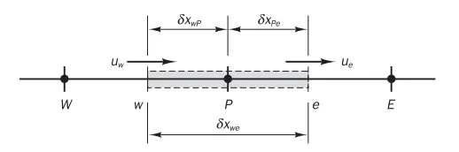
By integration of the above equation over the control volume gives,
`(rho*u*A)_e - (rho*u*A)_w = (alpha*A*(dT)/dx)_e - (alpha*A*(dT)/dx)_w`
for convenience we define
`F = rho*u` and `D = alpha/(deltax)`
assume `A_w = A_e = A`
The discretised equations are
`F_e*phi_e - F_w*phi_w = D_e*(phi_E - phi_P) - D_w*(phi_P - phi_W)`
Central differencing approach is used to represent the contribution of the diffusion terms.
Diffusion influences properties along its gradients in all directions, whereas convection spreads influence only in the flow direction.
This results into a limit on the grid size, which is dependent on the relative strength of convection and diffusion. Hence the need for interpolation schemes.
For the convective terms different interpolation schemes are used to compute the cell face values.
1) Central differencing scheme
2) Upwind differencing scheme
3) Hybrid differencing scheme
4) QUICK, TVD schemes
1)Central differencing scheme
The Cds uses linear interpolation to calculate the cell face value for the convective terms, it is a second-order accurate scheme.
`phi_e = (phi_P + phi_E)/2`
The Peclet number is defined as Pe = F/D, it is a measure of relative strength of convection and diffusion.
The Cds obeys the properties of conservativeness, but at Pe>2(convection dominates) it becomes unbounded and oscillates or produces 'wiggles' about the exact solution.
It also does not take into account the transportiveness or the direction of the flow or the strength of convection relative to diffusion.
2) Upwind differencing scheme
If the flow is strongly convective from west to east, the west cell face should receive stronger influence from node W than node P.
The Uds takes into account the flow direction when determinig the value at a cell face. The convected value at a cell face is taken to be equal to value at upstream node. It is only first-order accurate.
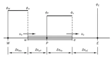
When the flow is in the positive direction, from west to east,
`phi_w = phi_W and phi_e = phi_P`
The Uds is conservative , bounded and shows trasnportiveness.
Its only drawback is it introduces false diffusion when the flow is not aligned with the grid lines.
3) Hybrid differencing scheme
Hybrid differencing scheme is based on Cds and Uds. The central differencing scheme which is 2nd order is employed for small Peclet number (Pe<2) and the upwind scheme which is 1st order accurate for large Peclet number (Pe>=2).
4)QUICK or Quadratic upwind differencing scheme
The QUICK scheme uses quadratic interpolation to obtain the face value of the convective terms.
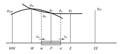
For example, when flow is from W to E, a quadratic fit through WW, W and P is used to evaluate `phi_w`. The QUICK scheme is conditionally stable.
The QUICK scheme is third-order accurate.
5)TVD scheme
The TVD schemes addresses the undesirable, oscillatory behavior of higher-order schemes. In TVD schemes, the tendency towards oscillation is countered by adding and artificial diffusion fragment towards upstream contribution.
The upwind differencing for the face value gives,
`phi_e = phi_P`
The linear upwind differencing(LUD) yields the following expression for `phi_e`
`phi_e = phi_P + (phi_P - phi_W)/2`
The LUD scheme can be thought as the sum of the basic UD flux plus an additional flux to improve order of accuracy.
The additional flux is written as a function `psi`.
`phi_e = phi_P + (0.5*psi(r))*(phi_E - phi_P)`
`psi(r)` is called the flux limiter function.
The flux limiter function constrains or limits the range of possible values of the additional convective flux which was introduced to make the scheme higher-order.