Week 2 - Flow over a Cylinder.

The flow past a cylinder for intermediate range of Reynolds number has analytical solution which are elusive or do not exist. The results are based on experimentation and numerical schemes. The observed phenomena are discussed in brief from small to high Reynolds number.

`Re = (rho*U_(infty)*d)/(mu)`

Low Reynolds number

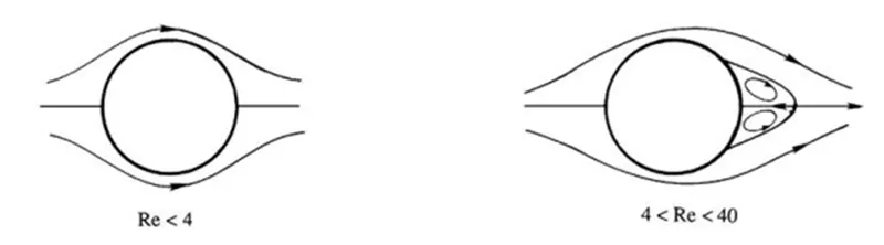
The creeping flow around a cylinder is characterized by Re < 1 , where `U_infty` is the upstream flow and d is the cylinder’s diameter. The flow generates a symmetrical pattern of streamlines.

For Re > 4 two small eddies appear behind the cylinder and a closed separation zone. The wake is completely laminar and the vortices rotate in a manner consistent with the external flow.

Moderate Reynolds number

As Re reaches 40, the wake behind the cylinder becomes unstable. For Re `approx`100, the wake develops a slow oscillation in which the velocity is periodic in time and down-stream distance, with the amplitude increasing downstream.

For 40<Re<80 the vortex street do not interact with the pair of attached eddies. As Re increases above 80, the vortex street forms close to the cylinder and the attached eddies begin to oscillate and periodically break of alternately from the two side of the cylinder.

The oscillating wake develops into two staggered rows of vortices with opposite sense of rotation. Von Karman studied the phenomenon and concluded that a non-staggered row is unstable and staggered is stable. Because of the similarity of the wake to footprints on a street, the staggered row of vortices behind a blunt body is called a von Karman vortex street.

While an eddy sheds on one side, that on the other side forms, which results in an unsteady flow near the cylinder. As vortices of opposite circulation are shed alternately, the cylinder experiences an oscillating lift or lateral force perpendicular to the upstream flow direction.

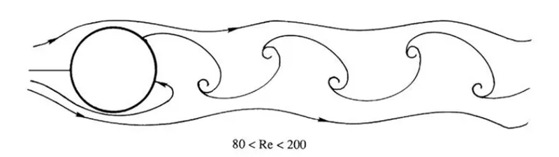
The passage of vortices cause velocity measurements in the cylinder’s wake to have a dominant periodicity and this frequency Ω is expressed as the Strouhal number,

`St = (Omega*d)/(U_infty)`

High Reynolds number

Above Re = 200, the vortex street becomes unstable and irregular, and the flow becomes chaotic. The wake may be described as fully turbulent several cylinder diameters downstream.

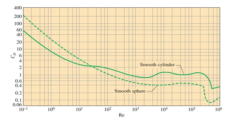
At high Reynolds number, the frictional effects upstream are confined near the surface. For Re < 3*10^5, the boundary layer is laminar, although the wake may be completely turbulent. The laminar boundary layer separates at = 82° from the forward stagnation point. The pressure in the wake downstream is constant and lower than upstream pressure. The drag in this Re range is primarily due to asymmetry of pressure distribution. The cylinder’s drag coefficient also stays constant at a value near unity.

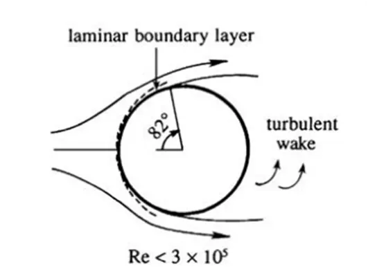
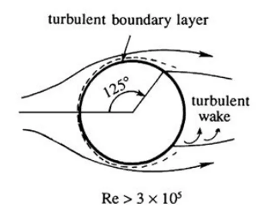
For `3*10^5 < Re < 3*10^6`, the laminar boundary layer becomes unstable and transitions to turbulence. Because of its greater average near-surface flow speed, a turbulent boundary layer is able to overcome a larger adverse-pressure gradient.

The turbulent boundary layer separates at 125° from forward stagnation point, resulting in thinner wake and in a pressure distribution similar to potential flow.

The drag coefficient also drops from 1.2 to 0.33. For values of `Re >3*10^6`, the separation point moves upstream as the Reynolds number increases, resulting in a mild increase of the drag coefficient.

Measured drag coefficient, `(C_D) vs. Re`

Since vortex shedding is a case of oscillating flow, resonance can occur if the frequency of vortex shedding is near a body’s structural vibration frequency. Electric transmission wires are prone to such phenomenon, which leads to singing of wires. Slender structures also flutter at critical wind speeds. Failure of the Tacoma suspension bridge was caused when wind vortex shedding caused resonance with torsional oscillations of bridge.

For this project, following are the objectives,

1. To perform steady and transient simulation of flow past a cylinder using Ansys Fluent.
2. To observe von Karman vortex street phenomenon.
3. To determine Strouhal number for steady and transient simulation at Re = 100.
4. Determine drag and lift coefficients for different Reynolds number regimes (for a steady flow simulation). Observe the variation of these force coefficients with respect to Reynolds number.
5. Creating a body-fitted mesh to accurately simulate the flow close to the wall of the cylinder.
6. Create a user-defined material, having defined properties such as density, dynamic viscosity.

MODELLING AND PROBLEM APPROACH

The model which will be simulated is a 2D rectangular control volume, with a cylinder of circular cross section, placed at a point. Since this is a 2D simulation, the depth of the cylinder is neglected. The model is created in SpaceClaim, using standard options. The inlet boundary is placed at 10*D (D is cylinder diameter) distance from the cylinder centre. The outlet boundary is at 40*D from the cylinder centre. The top & bottom boundaries are at 5*D distance from the cylinder centre. The pull tool is used to extrude the cylinder to create a single surface containing the cylinder and the control volume rectangle.

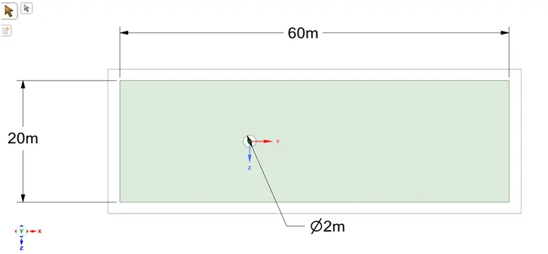
The boundaries of the control volume are

1. left-most inlet
2. right-most outlet
3. top & bottom symmetry
4. cylinder wall

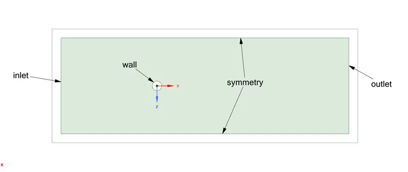
1. The model will be simulated using laminar flow model in Ansys Fluent for different Reynolds number.
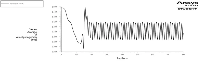
2. A monitor point is placed at a distance of four cylinder diameters from centre of the cylinder downstream of the flow. Since the velocity downstream oscillates due to the turbulent wake, its plot helps to determine whether the flow has reached steady state and the solution has converged or not. The magnitude of velocity at this point is monitored for each Reynolds number flow regime by plotting it against the number of iterations/flow time. Based on the plot, it will be decided whether the solution has converged or not.
3. For Re = 100, both steady and transient flows are simulated and the Strouhal number is determined for both.
4. Drag and lift coefficients are plotted separately different Reynolds number for a steady flow and will be compared with standard literature.

BOUNDARY CONDITIONS.

• The inlet will be a velocity-inlet, with the magnitude of velocity calculated according to the Reynolds number regime being considered. The outlet is a pressure-outlet, which is specified as the gauge pressure in Pa. Since the pressure is assumed to be atmospheric, gauge pressure is taken as 0 Pa.
• The cylinder wall is a stationary wall with the no-slip shear condition.
• The top & bottom walls are symmetry walls.

The laminar model in Ansys Fluent solves the continuity and the viscous Navier-Stokes equations.

`(delrho)/(delt) + (delrhou)/(delx) + (delrhov)/(dely) + (delrhow)/(delz) = 0`

`rho*(DvecV)/(Dt) = -vecgradP + rho*vecg + mu*grad^2vecV`

The solver is pressure-based solving either steady or transient equations for a planar surface. The SIMPLE algorithm is chosen as the solution method. Hybrid initialization is used to initialize the solution.

MESH

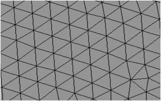
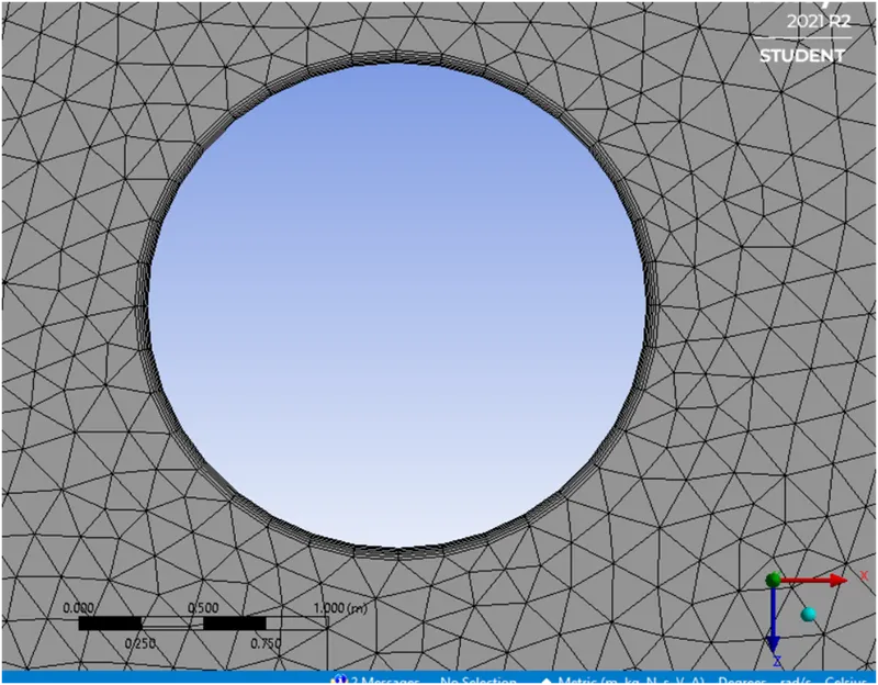
The meshing of the model is as shown (element size = 0.2m).

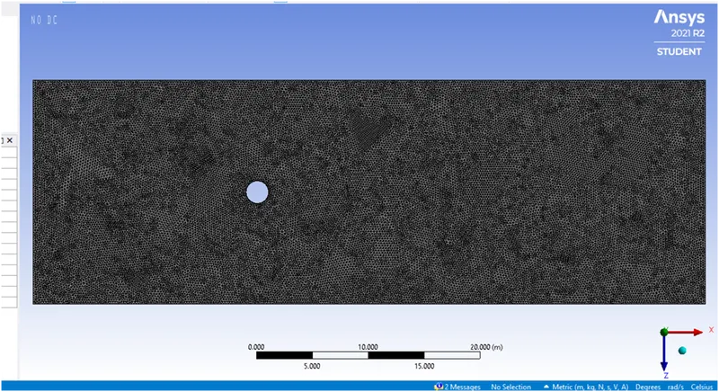
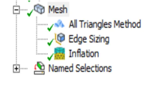
The mesh is generated using the following options,

Triangular element shape

The ‘All Triangles Method’ defines the mesh type as ‘Triangles’ for the surface of the model. The shape of the elements of the mesh is set to ‘Triangles’. An element size of 0.2m is chosen.

Edge sizing Inflation layer

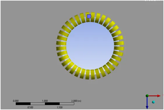
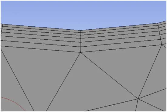
The ‘Edge sizing’ divides the cylinder wall into a number of divisions to make the mesh finer near the wall. ‘Inflation’ layer is added to the wall which is of 6 layers, having first layer thickness of 0.005 m, with a growth rate of 1.2. The inflation layer captures the boundary layer more accurately by stacking high aspect ratio elements in a direction normal to the flow.

Case 1: - The model is simulated for both steady and transient flow at Re = 100. The Strouhal number is determined for both.

`mu = 0.05 (kg)/(m s) " " Re = 100` diameter(d) = 2 m. From the above data the free stream velocity is `U_infty = 2.5 m/s`

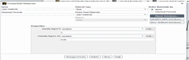
The user-material has the following properties

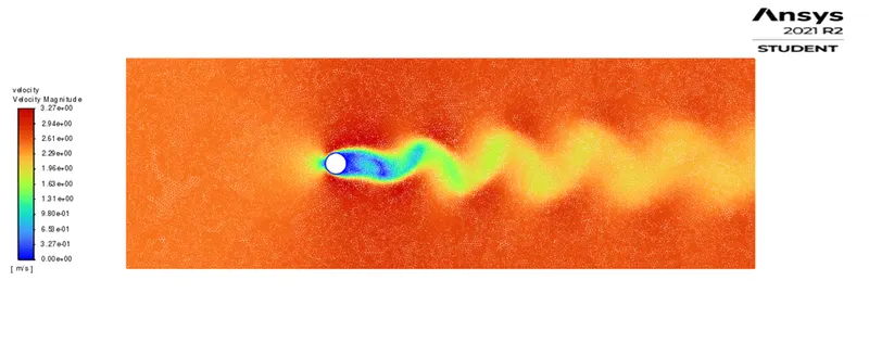
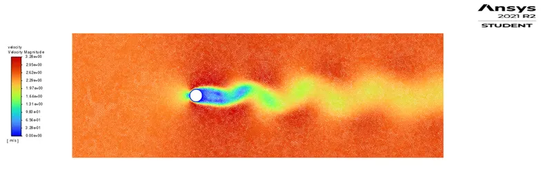
Velocity contour for

1. Steady 2. Transient

Pressure contour

1. Steady 2. Transient

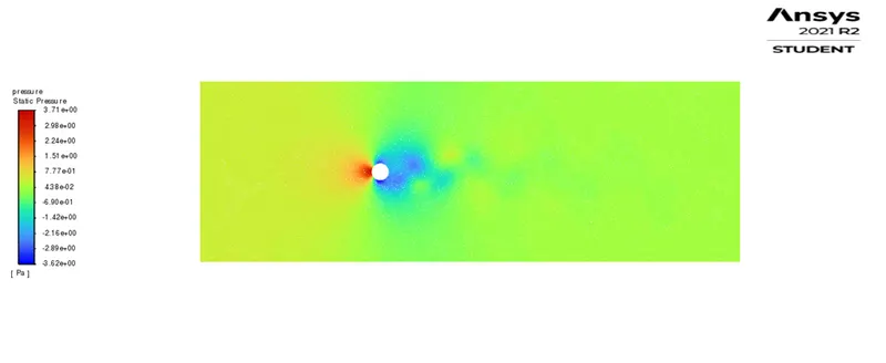
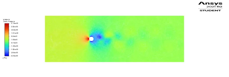
Monitor point velocity

1. Steady 2. Transient

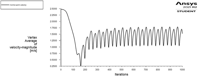
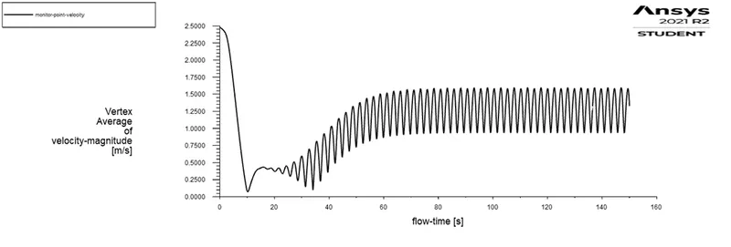
The coefficient of drag is determined by setting the reference values in Ansys accordingly.

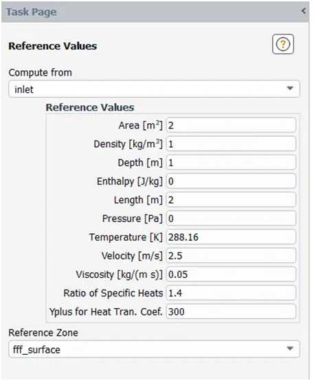
Compute from: - Refers to the boundary zones from which the reference values are defined. For this case the inlet boundary is chosen as the reference for free stream velocity.

Area: - The frontal/planform area which is used to calculate force coefficients i.e. lift and drag. Cylinder is a blunt body hence the frontal area is used which is a rectangle of width equal to diameter of cylinder.

Depth: - The reference depth for 2D volumes. It is set to 1m for this case.

Length: - The length over which the force coefficients will be computed.

Density & Viscosity: - The user-defined material values are chosen. For this case density = 1 kg/m^3 and viscosity = 0.05 kg/ (m s).

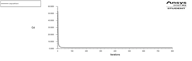
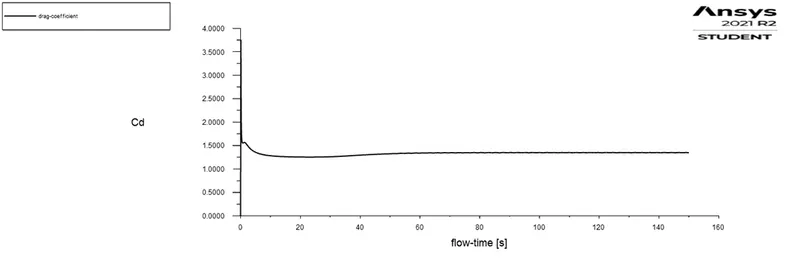
Coefficient of drag

1. Steady 2. Transient

Coefficient of lift

1. Steady 2. Transient

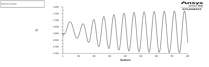
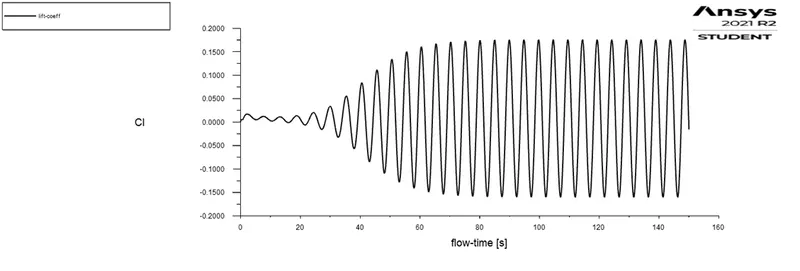
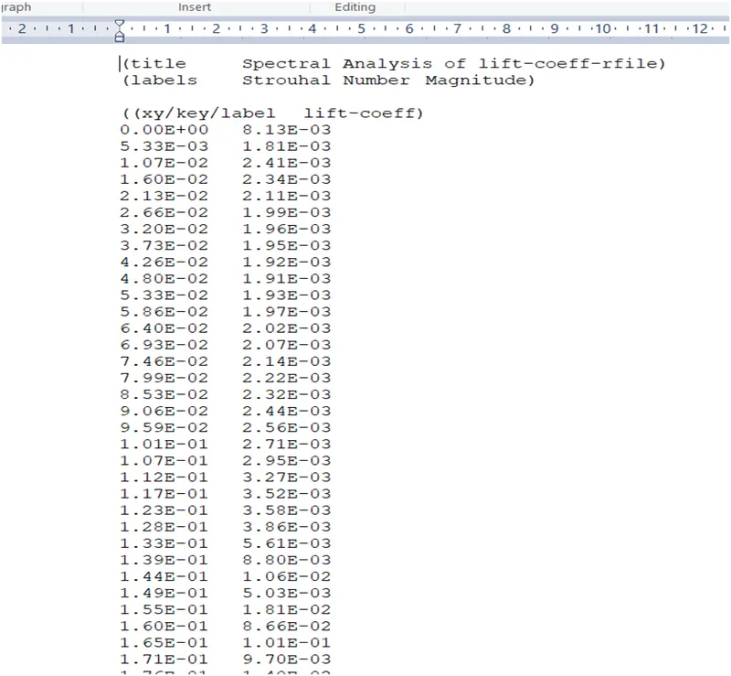
The Strouhal number is calculated by applying FFT to the coefficient of lift plot. From this we get a Strouhal no. v/s magnitude plot. The data for this plot is extracted as a CSV file which is parsed in Excel, Wordpad etc. For the maximum value of magnitude, the corresponding value of Strouhal number is the appropriate one.

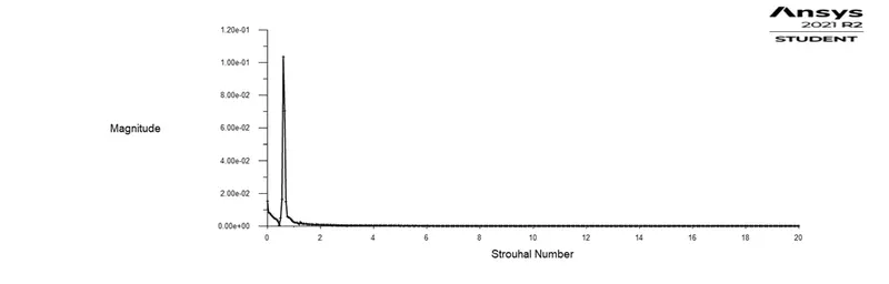
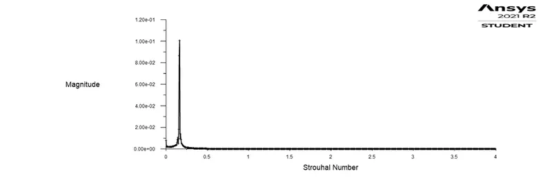
Strouhal number

1. Steady 2. Transient

Inferences

1. Strouhal number

1] Steady state = 0.6 2] Transient state = 0.17

2. The transient state Strouhal number = 0.17, is closer to the experimental value of 0.21.
3. It is visible from the velocity contours that the steady simulation has higher frequency of oscillations as compared to transient state.
4. The monitor point velocity oscillates uniformly about a particular value after certain amount of iterations or flow time has passed. We can conclude that convergence has been achieved at this state.

Case 2: - For case 2, we determine drag and lift coefficients for different Reynolds number regimes (objective 4). Re is set to 10, 100, 1000, 10000, 100000.

The Reynolds number can be changed by either changing the fluid viscosity or the free stream velocity. For this case, the latter is preferred. The dynamic viscosity is set to 0.001 m^2/s. Fluid density is set to 1 kg/m^3. The free stream velocity is calculated from the Reynolds number formula `Re = (rho*U_(infty) * d/mu)` ). The table below shows the results after the simulation is run for each of the Reynolds number. The drag and lift coefficient values are also mentioned in the table which were obtained from the simulation results.

`mu` = 0.001 m^s/s	Re	U	Cd	Cl
	10	0.005	3.332	-0.00037
	100	0.05	1.346	-0.0696
	1000	0.5	0.82459	-0.4955
	10000	5	1.2024	0.65
	100000	50	0.9466	0.559

A] For Re = 10, U = 0.005 m/s

Velocity contour Pressure contour

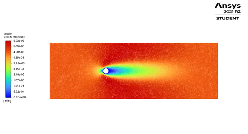
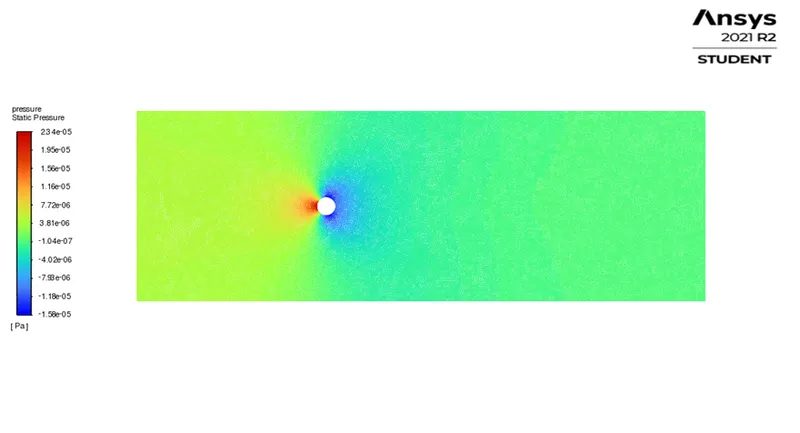
Monitor point velocity Residuals

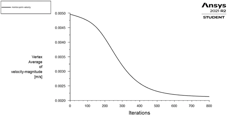
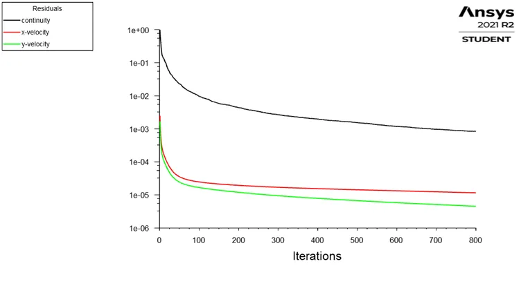
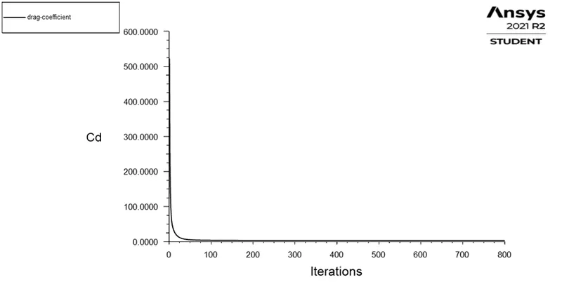
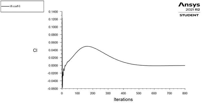
Drag coefficient Lift coefficient

Inferences

1. Drag coefficient Cd = 3.332, lift coefficient = -0.00037 (negative lift coefficient means the force is acting downwards as opposed to upwards.).
2. Drag forces are significant for this case. Lift is negligible.
3. Since Re < 40, the flow is in steady state and forms a symmetric wake region behind the cylinder.
4. The monitor point velocity decreases and approaches a constant value after 400 iterations. There are no observed oscillations of velocity at the monitor point.
5. The drag and lift coefficients approach a constant value after 400 iterations.

B] For Re = 100, U = 0.05 m/s

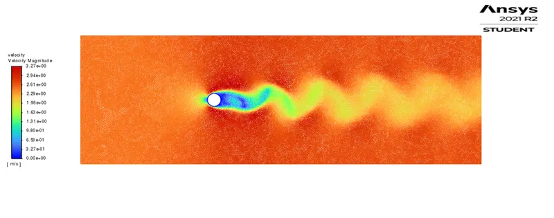
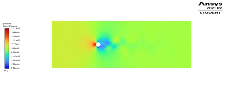
Velocity contour Pressure contour

Monitor point velocity Residuals

Drag coefficient Lift coefficient

Inferences

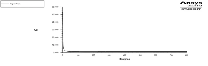
1. Drag coefficient = 1.346, lift coefficient = -0.0696
2. The drag coefficient reduces whereas the absolute value of lift coefficient increases.
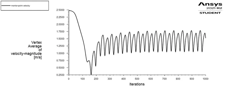
3. For Re = 100, the wake develops a slow oscillation. The velocity is periodic in time and the amplitude of oscillation increases downstream. The attached eddies break off periodically and alternately from the two sides of the cylinder.
4. The monitor point velocity starts to oscillate at about 160 iterations. The amplitude and the mean velocity of oscillation reach a steady state and the oscillations are uniform after some iterations.
5. The coefficient of drag also approaches a constant value.
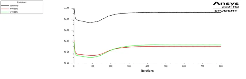
6. The uneven pressure distribution as seen in the pressure contour results in an oscillating lift or lateral force on the cylinder, which is confirmed by the oscillations of the lift coefficient.

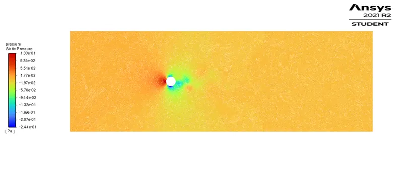
C] For Re = 1000, U = 0.5 m/s

Velocity contour Pressure contour

Monitor point velocity Residuals

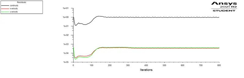
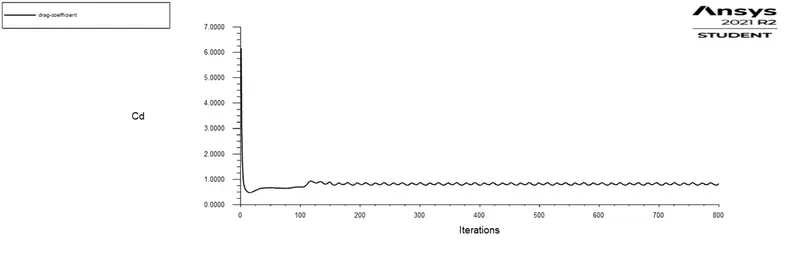
Drag coefficient Lift coefficients

Inferences

1. Drag coefficient = 0.82459, lift coefficient = -0.4955
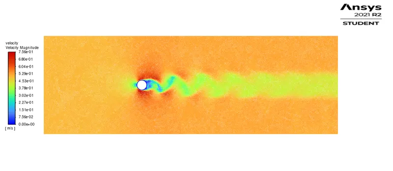
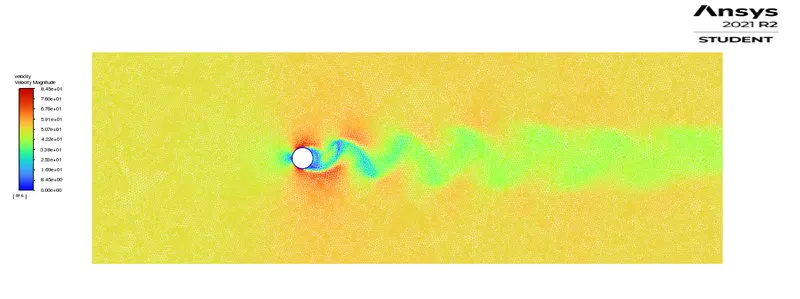
2. The wake has become fully turbulent which is visible from the velocity contour although the flow is laminar.
3. The drag coefficient has reduced significantly compared to previous values. The lift coefficient has also marginally increased. The lift force is still downwards. There are small oscillations in drag coefficient, which persist till the end of iterations

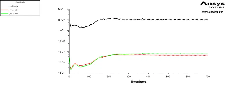
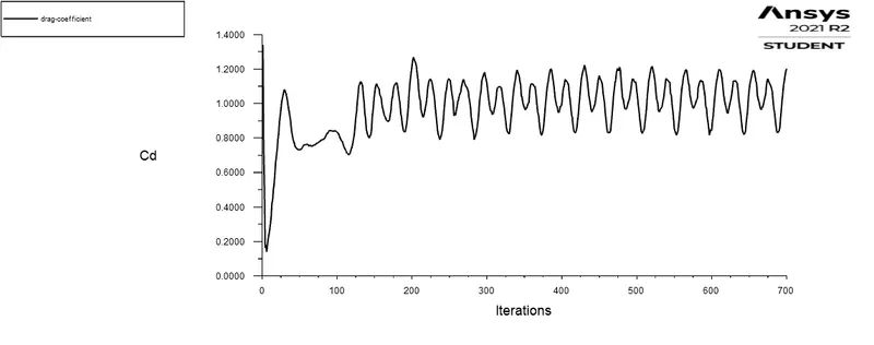
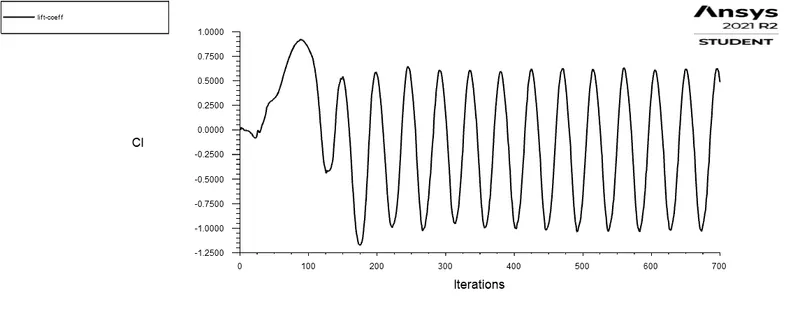
D] For Re = 10000, U = 5 m/s

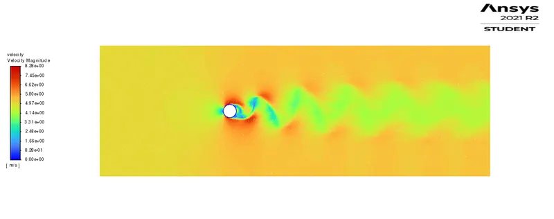
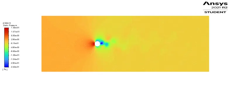
Velocity contour Pressure contour

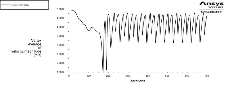
Monitor point velocity Residuals

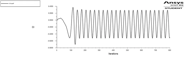
Drag coefficient Lift coefficient

Inferences

Drag coefficient = 1.2024, lift coefficient = 0.65

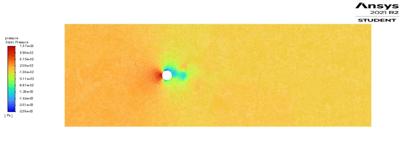
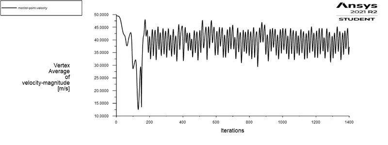
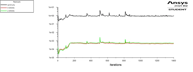
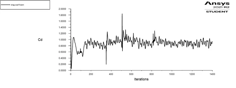
E] For Re = 100000, U = 50 m/s

Velocity contour Pressure contour

Monitor point velocity Residuals

Drag coefficient Lift coefficient

Inferences

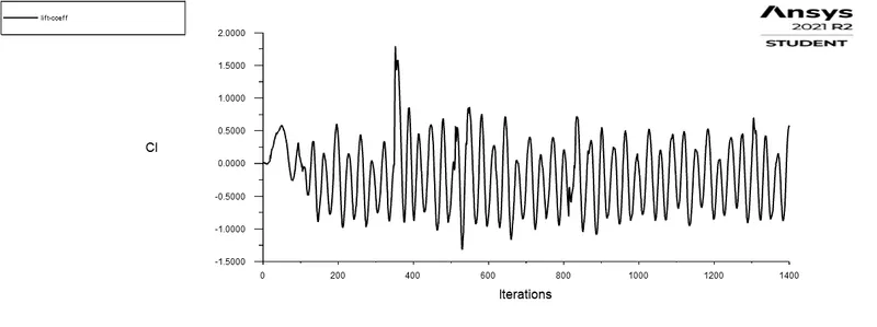
1. Drag coefficient = 0.9466, lift coefficient = 0.559
2. The oscillations in monitor point velocity show that the wake has become completely turbulent. The drag & lift coefficients also have random fluctuations.
3. The drag coefficient decreased marginally whereas the lift coefficient has increased.

COMPARISON WITH THEORETICAL VALUES

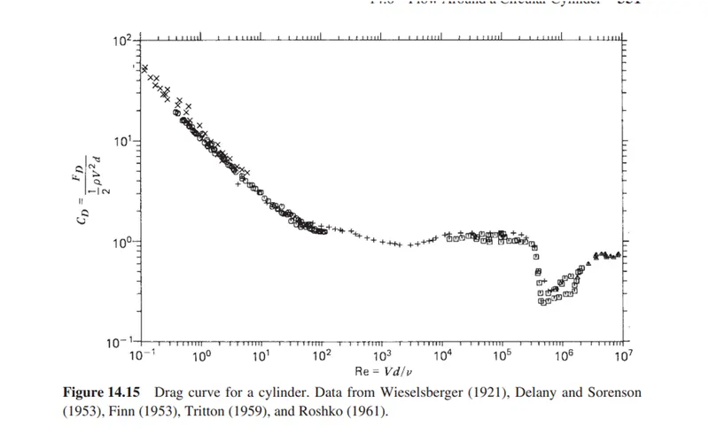
Plot of Cd v/s Re for a cylinder from the book ‘Incompressible flow (Wiley) by Ronald Panton’.

From the plot, the values of drag coefficient for Reynolds number of 10, 100, 1000, 10000, 100000 are as follows

Re	Cd
10	3.22
100	1.4
1000	0.94
10000	1.18
100000	1.01

The table for comparison of drag coefficient is shown below,

Re	U	Cd (simulation results)	Cd(theoretical results)	%difference
10	0.005	3.332	3.22	3.38
100	0.05	1.346	1.4	3.8
1000	0.5	0.83	0.94	11
10000	5	1.2024	1.18	1.9
100000	50	0.95	1.01	5.94

It can be concluded that as the Reynolds number decreases significantly between 10<Re<1000 but remains close to 1 between 1000<Re<100000.

Reference material : -

1) Fluid mechanics - Fundamentals & applications by Cengel & Cimbala.

2) Incompressible flow (Wiley) by Ronald Panton.