Week 4 - CHT Analysis on Exhaust port

INTRODUCTION

Conjugate heat transfer involves a combination of heat transfer in solids and heat transfer in fluids. In solids conduction is dominant whereas in fluids convection.

In most cases, heat transfer in solids is due to conduction. Fourier’s law of heat conduction defines the conductive heat flux proportional to the temperature gradient. `q = -k*nablaT`

For fluids, the contributions for heat equation include,

• Transport of fluid implies energy transfer, which is the convective contribution.
• Viscous effects produce fluid heating.
• As fluid density is temperature-dependent, pressure work contributes to heat equation. Example: - compressing air produces heat.

Newton’s law of cooling governs the convection heat transfer. According to Newton’s law of cooling, rate of heat loss is directly proportional to the temperature difference between the two interacting bodies.

`Q = h*A*DeltaT`

h is the heat transfer coefficient in (W/(m^2-K). It depends on the flow regime and the fluid physical properties. Is not a system property and must be found experimentally.

Conjugate heat transfer analysis can accurately predict heat transfer by simultaneously solving the relevant solid and fluid flow heat transfer equations using a computer. For example: - conduction through solids, free and forced convection in gases/fluids and thermal radiation.

CHT analysis is beneficial where heat transfer is either non-uniform or difficult to calculate empirically. Local variation of wall heat transfer coefficients are directly calculated within the model rather than based on empirical calculations.

Applications include heat exchangers, electronic equipment, cooling and heating systems.

The exhaust manifold is used in a car or truck’s exhaust system. It connects the exhaust port on each cylinder to a common exhaust pipe. The exhaust manifold is designed in such a way that it expels as much exhaust from the cylinder as possible.

The exhaust manifold acts as a funnel that concentrates and then uses exhaust pressure to expel gases with force to exit the system.

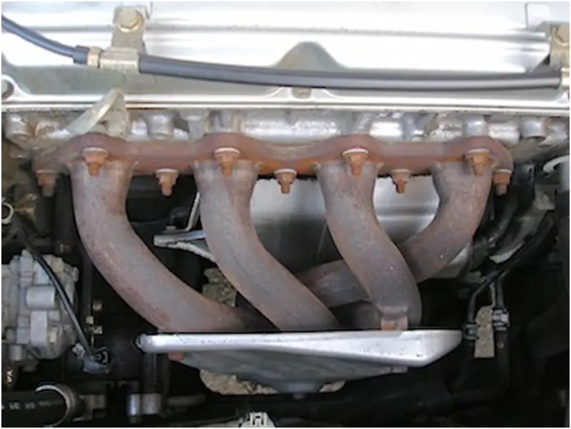
The exhaust gases which are generated after the combustion of the air-fuel mixture in an engine are at a high temperature which might be of the order of several hundred degrees Celsius. When these exhaust gases enter the exhaust manifold, they exchange energy with the exhaust manifold in the form of heat transfer. The mode of heat transfer from the hot gases to the solid manifold body is forced convection, while the heat transfer within the solid body is by conduction. The CHT analysis of exhaust manifold helps in analyzing the following: -

• Temperature distribution
• Heat flux rate analysis – calculation of wall heat flux rates or heat transfer coefficient.
• Heat transfer coefficient analysis.
• Thermal analysis

MODELLING

The model for this case will be simulated in Ansys Fluent, which solves the fluid continuity, momentum as well as the energy equation.

Continuity `nabla.V = 0`

Momentum `rho(dV)/(dt) = rhog - nablap + munabla^2V`

Energy `rhoC_p(dT)/(dt) = knabla^2T + Phi`

The boundary conditions for these equations are as follows: -

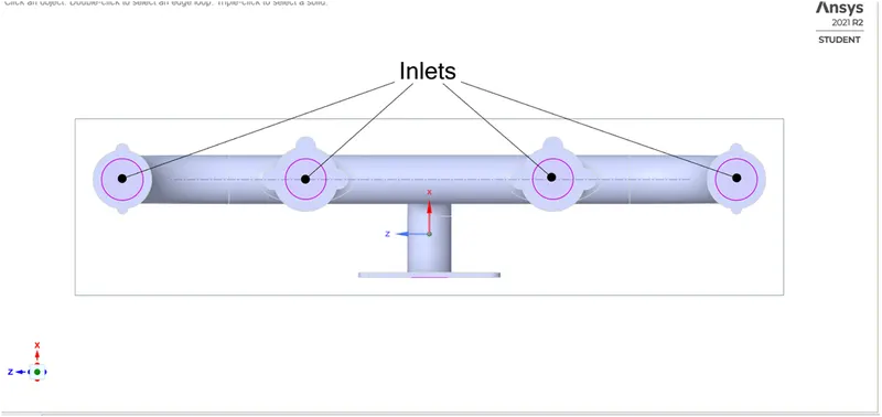
• Inlet: - velocity inlet
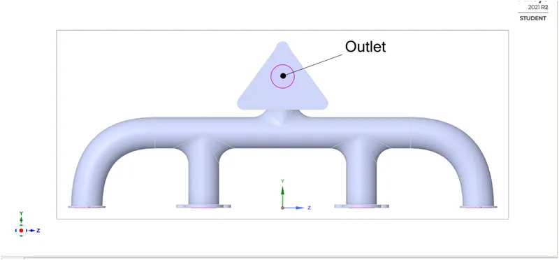
• Outlet: - pressure outlet
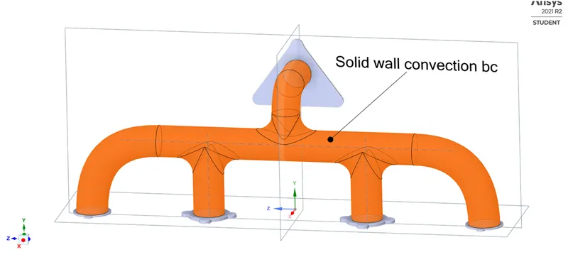
• Solid wall: - convection

To determine the heat transfer coefficient, there are two approaches

• Wall heat transfer coefficient
• Surface heat transfer coefficient

The near-wall region has either a linear viscous sub-layer or a wall function defined by the turbulence model. Which means that more refined the mesh near walls, more accurate will be the HTC. This is because the heat transfer coefficient is determined according to the equation

`h = q/(T_(reference) - T_(wall))`

The Tref is the reference temperature which the solver chooses to calculate the HTC. The solver chooses the Tref from the cell centroid which is nearest to the wall. This approach will involve a finer mesh, more computational time & resources.

Either this or we can input the Tref or reference temperature ourselves in the ‘Reference Values’ options in Ansys Fluent. The reference temperature will be the free stream temperature at the inlet.

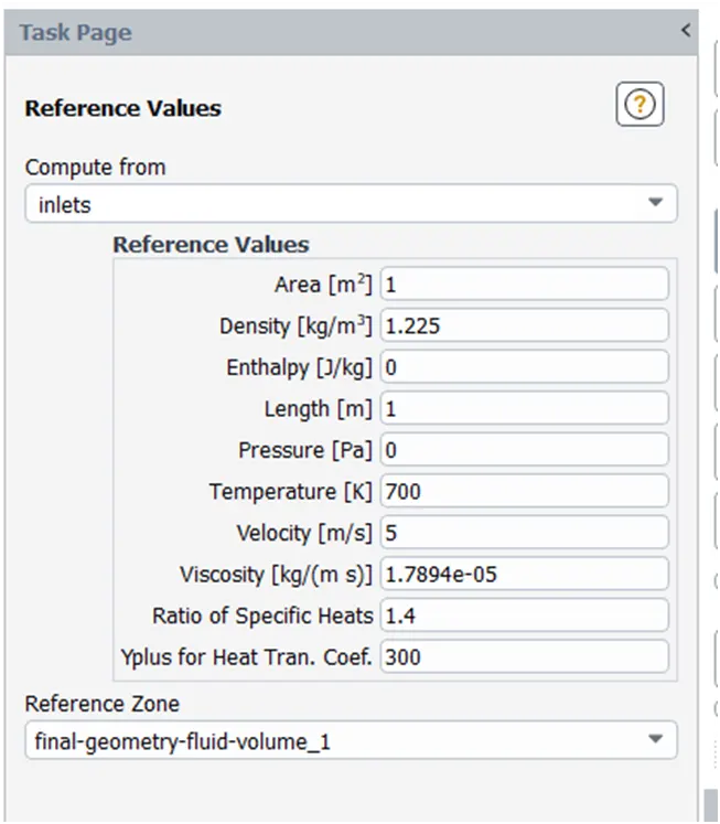
In this way we calculate the ‘Surface heat transfer coefficient’.

SOLVER REQUIREMENTS

The Reynolds number is given by

`Re = rho*U_infty*D/mu`

For this case `rho` = 1.225 kg/m^3

`U_infty` = 5 m/s

D = 0.170 m

`mu` = 1.78943e-05 kg/(m-s)

Re = 58,189.896

The flow is turbulent and a suitable turbulent model is to be chosen. For this case, the k-epsilon(`k-epsilon`) model with standard wall function is chosen. This model is suitable for fully developed high Reynolds number flows. The near-wall treatment is done using the wall functions which employ an empirical relation for the velocity profile near-wall.

The y+ value for the k-epsilon model should not be less than 11, since it affects the solution’s accuracy below this value.

`rho` = 1.225

Re = 58,189.896

Y+ = 120 = y.u*/nu

U* = sqrt(tauw/rho)

`tau_w` = ½.Cf.rho.(`U_infty`^2)

Cf = 0.0576.(Re^1/5) = 0.51688

`tau_w`= 7.9147 Pa

U* = 2.5418 m/s

Y+ = 120 = y.(2.5418)/1.4607e-05

Y = 0.68962mm is the first layer thickness for the inflation layer. For a growth rate of 1.2 and a total of 5 layers, the total thickness is calculated as

y+ = 120	layer no	layer thickness in mm
	1	0.68962
	2	0.827544
	3	0.9930528
	4	1.19166336
	5	1.429996032
	Total thickness	5.131876192

Turbulence model: - k-epsilon

Near-wall treatment: - Standard wall function

Solution methods: -

Pressure Velocity Coupling

Scheme: - SIMPLE

GEOMETRY & MESH

The geometry of the exhaust manifold is as shown below; it has four inlets which connect to the exhaust port of the engine cylinder block and one outlet which connects to the exhaust pipe.

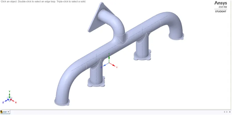
The geometry is divided into two parts: 1. Solid volume 2. Fluid volume, for the sake of convenience of meshing and defining boundary conditions. This is done using the volume extract option in SpaceClaim.

The solid volume is the outer pipe volume, whereas the fluid volume is the inner volume except the outer walls.

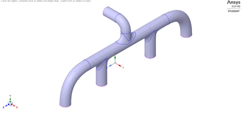
Fluid volume

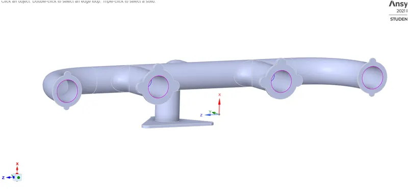
Solid volume

The mesh created is as follows

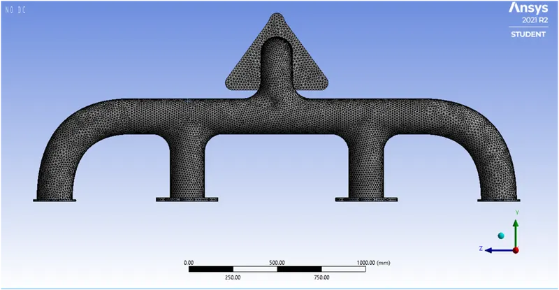
In addition to the default mesh, inflation layers for the fluid volume and a body sizing is added for the solid wall.

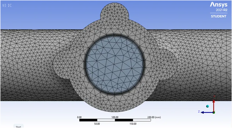
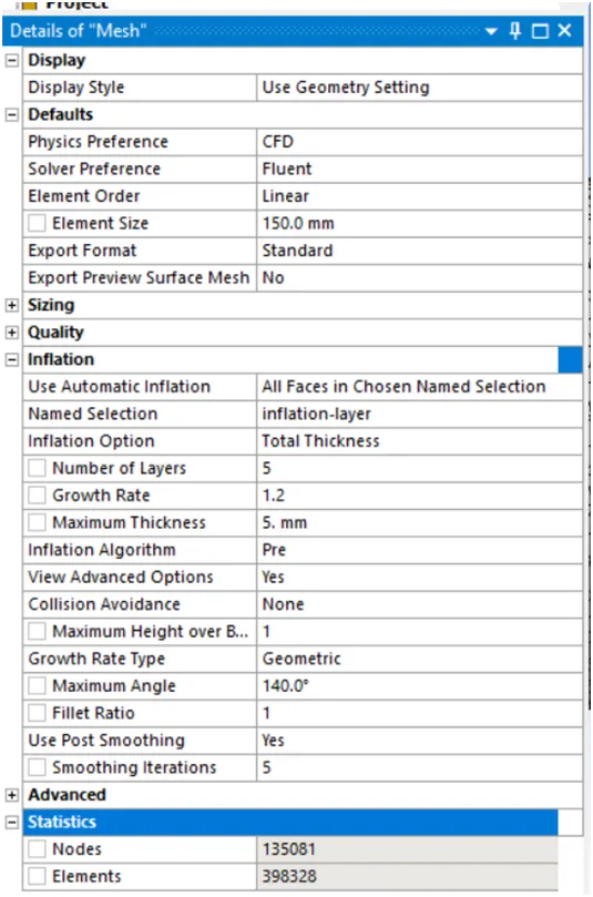
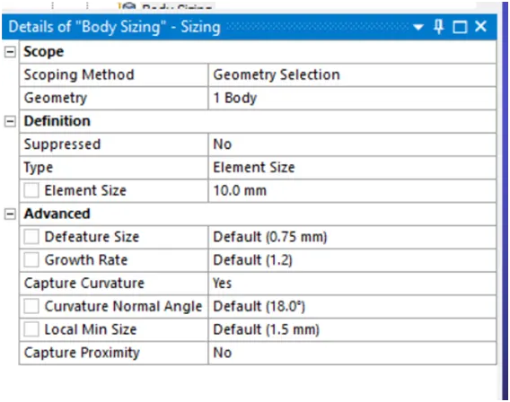
The mesh transition from the fluid volume to the solid volume is smooth and there are no overlaps between them. This is achieved by using the ’Share coincident topology’ option in SpaceClaim which enables the topology to be shared between two interfaces which in this case are the solid & the fluid volume. The inflation layer thickness is calculated based on the y+ value.

• The default mesh size is 150 mm.
• Inflation layers, layers 5, total thickness 5 mm, growth rate 1.2.
• Body sizing 10 mm.

RESULTS

For the boundaries the conditions are

• Inlet: - Velocity = 5 m/s; Temperature = 700 K
• Outlet: - Pressure(gauge) = 0 Pa
• Outer wall: - Convection BC HTC = 20 W/(m^2-K)
• Solid wall: - Adiabatic BC Heat flux = 0 W/m^2

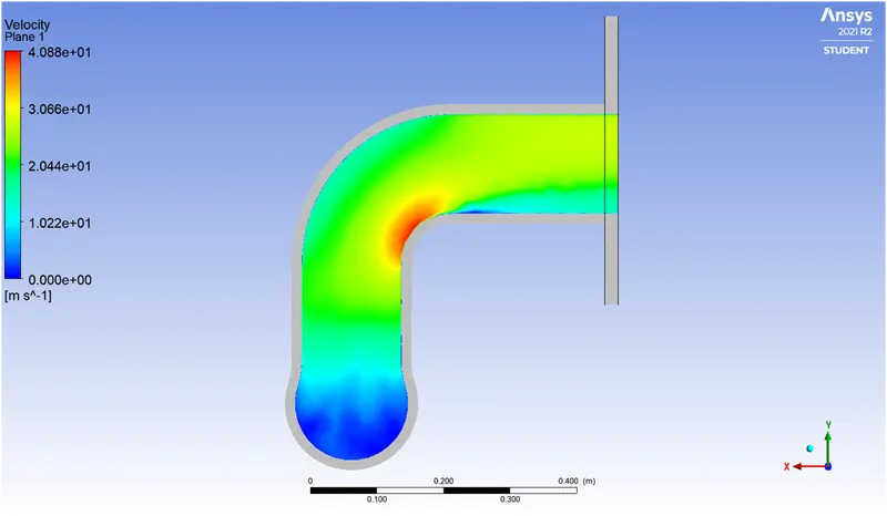
Velocity contour

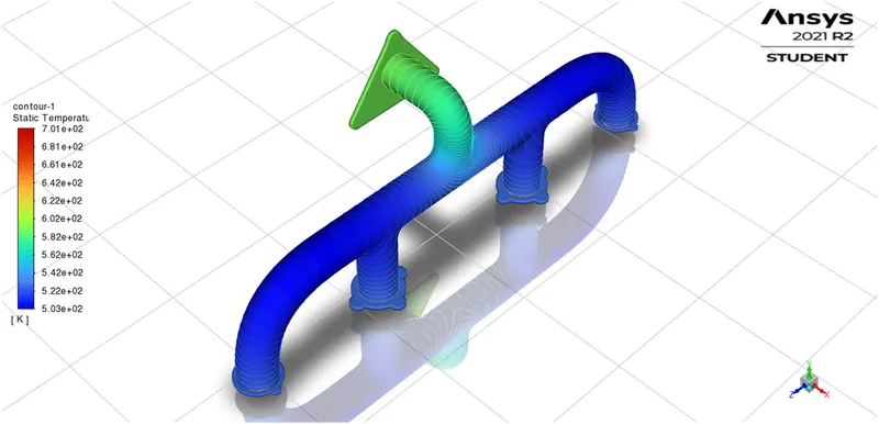
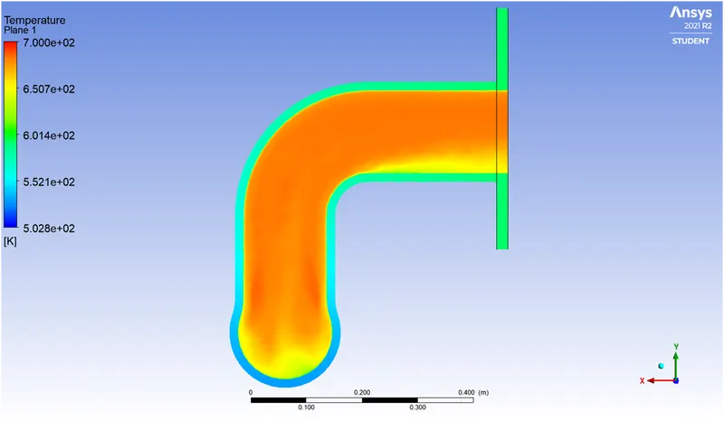
Temperature contours

At the outlet elbow.

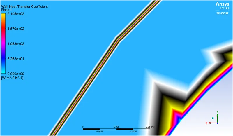
Wall HTC

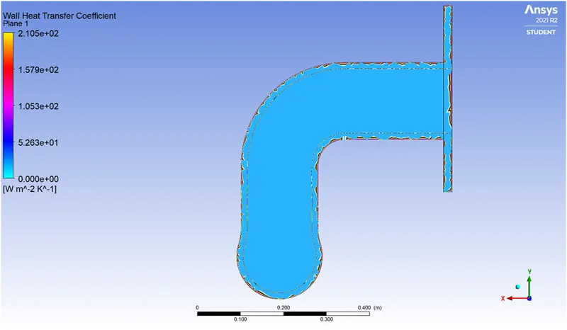
Close-up view of Wall HTC plot

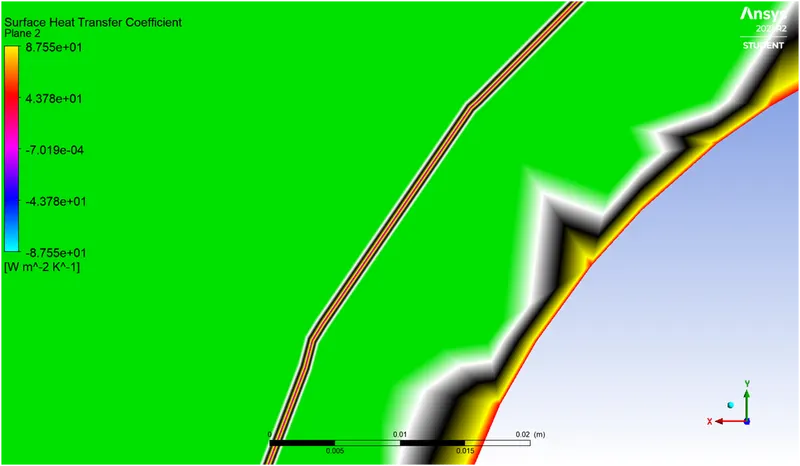
Close-up view of Surface HTC plot

INFERENCES

• The mass-flow from all the inlets converges at a single location near the outlet. Due to continuity, the flow accelerates. Around the elbow of the outlet, the flow accelerates and achieves the maximum velocity at the bend.
• The Reynolds number is also high in this region. The Nusselt number is related to the Reynolds & the Prandtl number by the relation.
• `Nu = 0.664*Re^0.5*Pr^0.33`
• The heat transfer coefficient is related to the Nusselt number by
• `h = Nu*k/l`
• As Re is high in this region, the Nusselt number increases which increases the heat transfer coefficient.
• Hence heat transfer coefficient is maximum here.

• The area-weighted average of the surface HTC is 26.288827 W/(m^2-K)

Wall htc = 210.52 W/(m^2-K)

Surface htc = 87.5528 W/(m^2-K)

• To verify the HTC predictions from simulation, we need experimental data from research papers or exhaust system manufacturing companies. The empirical relations are developed for a flat plate and only serve as an equation that explains the behaviour of the heat transfer coefficient.
• The accuracy of the prediction depends crucially on the size of the first grid/cell near the wall. The solver chooses the Tref at the nearest cell centroid. This Tref is used to calculate the HTC. Hence, the HTC is grid-dependent.
• The second approach is to use a prescribed Tref value, in this case the free-stream inlet temperature of 700 K is used.
• Both the approaches might result into a different HTC values.
• However, the first approach is more accurate but requires a finer mesh & high cell count.