Week 7 - Simulation of a 1D Super-sonic nozzle flow simulation using Macormack Method
The flow through a convergent divergent nozzle is assumed to be a steady, isentropic flow. At the inlet to the nozzle we have a reservoir, whose cross section area is very large. Hence the velocity at the inlet is very small, the properties at the inlet, pressure and temperature are stagnation properties.
The flow expands isentropically in the nozzle to supersonic speeds at the nozzle exit.
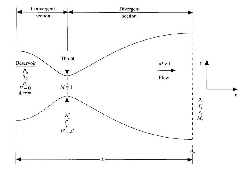
The flow is subsonic in the convergent section, sonic at the throat and supersonic in the divergent section.
The flow properties are uniform across a cross section. Although the area changes as a function of distance along the nozzle, x, therefore in reality the flow is two-dimensional. We assume that the flow properties vary only with x. Hence, called quasi-one- dimensional.
Analytical solution
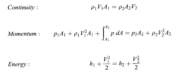
The flow through a nozzle is governed by the continuity, momentum and energy equations. For quasi-one-dimensional steady, isentropic flow they can be expressed as,
In addition to these, the variation of Mach number and other flow field variables along the nozzle length, are given as
The results are visualized as,
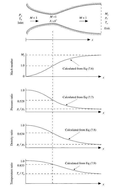
The flow through a nozzle does not happen by itself, it requires a pressure ratio between the exit and inlet, to accelerate the gas through the nozzle.Its variation is shown. It is usually applied as a boundary condition.
Numerical solution
1) The governing flow equations are partial differential equations, suitable for time marching solutions.
2) MacCormack's technique will be applied to this problem using finite-difference expressions.
3) The time-step and boundary conditions are choosen accordingly.
1)Non-conservative form
The nondimensionalized governing equations for the flow field are,



All the dashed variables refer to nondimensionalized values, refernced to reservoir values, they all vary between 0 and 1.
The above mentioned equations are then discretized into finite difference equations and then solved using MacCormack's method, which follows a predictor-corrector technique. In time marching solution, we know field variables at 't' and use them to determine values at 't +`Deltat`.
For the predictor step, we first determine the time derivative in the above equations, using forward differences for the spatial derivatives.

Then we find the predicted values of the variable `rho`,
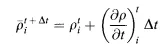
Now, we have predicted quantities at 't +`Deltat`.
Next, for the corrector step, we determine time derivative for 't +`Deltat`, using rearward differences for spatial derivatives and using the predicted quantity.
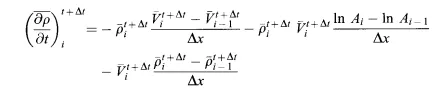
Now we determine the average time derivative,
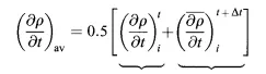
Finally, we have the corrected values of the variable `rho`,
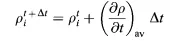
we find the other variables V, T in a similar fashion.
Time step :- The time step for the governing equations, has a stability constraint, given by
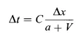
C is the Courant number, a the sonic velocity, V flow velocity, Deltax spacing between grid points.
since the sonic and flow velocity are varying along x, we determine the timestep for all grid points and then choose the minimum value.

Boundary conditions :- Our domain of study consists of two boundary points along the grid, 1 and N. 1 refers to inflow, N to outflow. Point 1 is essentially the reservoir, the inflow for the nozzle. Though the reservoir values do not change over time, the flow velocity at inflow is very low, it is not zero, if it were, then we wouldn't have any flow taking place. Though the reservoir has infinite area, we are starting at point 1, which has a finite area. Hence, 1 does not exactly correspond to the reservoir. Further, the characterisitic lines for the domain are as follows,
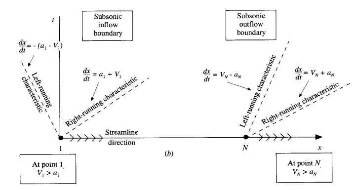
At the inlet one characteristic goes into the domain whereas one goes out to the left, at the outlet both the characteristics are propagating out of the domain.
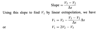
Hence we float one variable, V at the inlet. Using linear interpolation, we determine V at 1 using internal grid points,
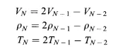
At the outflow, we float all flow field variables and determine them using linear interpolation,
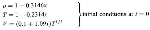
Nozzle shape and initial conditions :The initial conditions are choosen such that they are close to a steady state answer. If initial conditions are far from steady state, large gradients are formed, which can cause the solution to go unstable.
The nozzle shape is,

2) Conservative form
The conservative form differs from nonconservative in that, the conservative form contains primitive variables inside the partial derivatives whereas nonconservative has them outside the deivatives. This makes no difference for analytical solution and both are identical, whereas for numerical solution it is slightly different.
Continuity equation
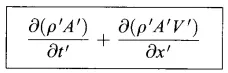
Momentum

Energy

Code for non-conservative
clear all
close all
clc

n = 31;
nt = 1400;
x = linspace(0,3,n);
dx = x(2) - x(1);

[nc_MF,nc_p,nc_M,nc_v,nc_rho,nc_t,nc_rho_th,nc_t_th,nc_time,nc_p_th,nc_M_th] = nonconservative(n,nt,x);


%plotting values at throat
ttotal = sum(nc_time);
f1 = figure(1);
f1 .WindowState = 'Maximized';
subplot(4,1,1)
plot(nc_rho_th,'r','Linewidth',1.5);
title('throat density')
grid on ;
subplot(4,1,2)
plot(nc_t_th,'g','Linewidth',1.5);
title('throat temperature')
grid on;
subplot(4,1,3)
plot(nc_p_th,'b','Linewidth',1.5);
title('throat pressure')
grid on;
subplot(4,1,4)
plot(nc_M_th,'y','Linewidth',1.5);
title('throat Mach number')
grid on;


%variation of flow variables along the x-direction
f2 = figure(2);
f2 .WindowState = 'Maximized';
subplot(4,1,1)
plot(x,nc_rho,'r','Linewidth',1.5);
title('density')
grid on;
subplot(4,1,2)
plot(x,nc_t,'g','Linewidth',1.5);
title('temperature')
grid on;
subplot(4,1,3)
plot(x,nc_p,'b','Linewidth',1.5);
title('pressure')
grid on;
subplot(4,1,4)
plot(x,nc_M,'y','Linewidth',1.5);
title('Mach number')
grid on;


%variation of mass flow rate
f3 = figure(3);
f3 .WindowState = 'Maximized';
plot(x,nc_MF(1,:),'r','Linewidth',1.5);
hold on
plot(x,nc_MF(50,:),'y','Linewidth',1.5);
hold on
plot(x,nc_MF(700,:),'b','Linewidth',1.5);
hold on
plot(x,nc_MF(100,:),'g','Linewidth',1.5);
title('mass flow rate at different timesteps')
legend('0delt','50delt','700delt','100delt')
grid on;

function [MF,p,M,v,rho,t,rho_th,t_th,time,p_th,M_th] = nonconservative(n,nt,x)

%inputs
n = 31;
x = linspace(0,3,n);
dx = x(2) - x(1);
gamma = 1.4;

%initial profiles
rho = 1 - 0.3146*x;%density
t = 1- 0.2314*x; %t: temperature
v = (0.1 + 1.09*x).*t.^0.5;
a = 1 + 2.2*(x-1.5).^2;%area

p = rho.*t;
M = v./(t.^0.5);
MF = rho.*a.*v;

%time steps
nt = 1400;
C = 0.5;

%outer time loop

tic
for k = 1:nt

    Dt = min((C*dx)./((t.^0.5) + v));
    rho_old = rho;
    t_old = t;
    v_old = v;
    p_old = p;
    M_old = M;
    %predictor step

    for j = 2:n-1

       dvdx = (v(j+1)-v(j))/dx;
       drhodx = (rho(j+1) - rho(j))/dx;
       dtdx = (t(j+1)-t(j))/dx;
       dlogadx = (log(a(j+1))-log(a(j)))/dx;

       %continuity equation
       drhodt_p(j) = -rho(j)*dvdx - rho(j)*v(j)*dlogadx - v(j)*drhodx;

       %momentum equation
       dvdt_p(j) = -v(j)*dvdx - (1/gamma)*(dtdx + (t(j)/rho(j))*drhodx);

       %energy equation
       dtdt_p(j) = -v(j)*dtdx - (gamma-1)*t(j)*(dvdx + v(j)*dlogadx);


       %updating values
       rho(j) = rho(j) + drhodt_p(j)*Dt;
        v(j) = v(j) + (dvdt_p(j))*Dt;
       t(j) = t(j) + dtdt_p(j)*Dt;

    end

    %corrector step
    for j = 2:n-1

       dvdx = (v(j)-v(j-1))/dx;
       drhodx = (rho(j) - rho(j-1))/dx;
       dtdx = (t(j)-t(j-1))/dx;
       dlogadx = (log(a(j))-log(a(j-1)))/dx;

       %continuity equation
       drhodt_c(j) = -rho(j)*dvdx - rho(j)*v(j)*dlogadx - v(j)*drhodx;

       %momentum equation
       dvdt_c(j) = -v(j)*dvdx - (1/gamma)*(dtdx + (t(j)/rho(j))*drhodx);

       %energy equation
       dtdt_c(j) = -v(j)*dtdx - (gamma-1)*t(j)*(dvdx + v(j)*dlogadx);

    end
    %compute average time derivative
    dvdt = 0.5*(dvdt_p + dvdt_c);
    drhodt = 0.5*(drhodt_p + drhodt_c);
    dtdt = 0.5*(dtdt_p + dtdt_c);

    %update final solution
    for i = 2:n-1
        rho(i) = rho_old(i) +drhodt(i)*Dt;
        v(i) = v_old(i) + dvdt(i)*Dt;
        t(i) = t_old(i) + dtdt(i)*Dt;

    end
    %apply boundary conditions
    %inlet
    v(1) = 2*v(2) - v(3);

    %outlet
    v(n) = 2*v(n-1) - v(n-2);
    rho(n) = 2*rho(n-1) - rho(n-2);
    t(n) = 2*t(n-1) - t(n-2);

    %variables

         p = rho.*t; %pressure
        M = v./(t.^0.5); %Mach number
        MF(k,:) = rho.*a.*v; %mass flow rate


    %Values at the throat
    rho_th(k) = rho(16);
    t_th(k) = t(16);
    v_th(k) = v(16);
    p_th(k) = rho(16).*t(16);
    M_th(k) =v(16)./(t(16).^0.5);
    time(k) = toc;

end


end
Code for conservative
clear all
close all
clc

n = 31;
nt = 1400;
x = linspace(0,3,n);
dx = x(2) - x(1);

[cMF,cp,cM,cv,crho,ct,crho_th,ct_th,cp_th,cM_th] = conservative(n,nt,x);

%time-wise variation of primitive variables
f1 = figure(1);
f1 .WindowState = 'Maximized';
subplot(4,1,1)
plot(crho_th,'r','Linewidth',1.5);
title('Time-wise variation of flow variables inside the nozzle for conservative form')
legend('Throat density')
xlabel('Number of timesteps')
ylabel('rho/rho0')
grid on ;
subplot(4,1,2)
plot(ct_th,'g','Linewidth',1.5);
legend('throat temperature')
xlabel('Number of timesteps')
ylabel('t/t0')
grid on;
subplot(4,1,3)
plot(cp_th,'b','Linewidth',1.5);
legend('throat pressure')
xlabel('Number of timesteps')
ylabel('p/p0')
grid on;
subplot(4,1,4)
plot(cM_th,'y','Linewidth',1.5);
legend('throat Mach number')
xlabel('Number of timesteps')
ylabel('M/M0')
grid on;


%variation of flow variables along the x-direction
f2 = figure(2);
f2 .WindowState = 'Maximized';
subplot(4,1,1)
plot(x,crho,'r','Linewidth',1.5);
title('Variation of flow variables inside the nozzle for conservative form')
legend('density')
xlabel('x along nozzle length')
ylabel('rho/rho0')
grid on;
subplot(4,1,2)
plot(x,ct,'g','Linewidth',1.5);
legend('temperature')
xlabel('x along nozzle length')
ylabel('t/t0')
grid on;
subplot(4,1,3)
plot(x,cp,'b','Linewidth',1.5);
legend('pressure')
xlabel('x along nozzle length')
ylabel('p/p0')
grid on;
subplot(4,1,4)
plot(x,cM,'y','Linewidth',1.5);
legend('Mach number')
xlabel('x along nozzle length')
ylabel('M/M0')
grid on;


f3 = figure(3);
f3 .WindowState = 'Maximized';
plot(x,cMF(nt,:),'r','Linewidth',1.5);
grid on;

function [MF,p,M,v,rho,t,rho_th,t_th,p_th,M_th] = conservative(n,nt,x)


n = 31;
nt = 1400;
x = linspace(0,3,n);
dx = x(2) - x(1);
a = 1 + 2.2*(x-1.5).^2; %area
gamma = 1.4;
C = 0.5;


for r = 1:n

if r >= 1 && r <= 6
 rho(r) = 1 ; %n = 1:6
 t(r) = 1;

elseif r >= 6 && r <= 16
  rho(r) = 1 - 0.366*(x(r)-0.5); %n = 6:16
  t(r) = 1- 0.167*(x(r) - 0.5);


elseif r >= 16 && r <= 31
rho(r) = 0.634 - 0.3879*(x(r) - 1.5); % n = 16:31
t(r) = 0.833 - 0.3507*(x(r) - 1.5);

end

end
v = 0.59./(rho.*a);

U1 = rho.*a;
U2 = rho.*a.*v;
U3 = U1.*((t./(gamma-1)) + (gamma/2).*(v.^2));
Dt = min(C.*(dx./((t.^0.5) + v)));

for i = 1:nt


   %Dt = min(C.*(dx./((t.^0.5) + v)));
   U1old = U1;
   U2old = U2;
   U3old = U3;

   F1 = U2;
   F2 = (U2.^2./U1) + ((gamma-1)/gamma)*(U3 - (gamma/2)*(U2.^2./U1));
   F3 = ((gamma.*U2.*U3./U1) - (gamma.*(gamma-1)/2).*(U2.^3./U1.^2));
   for m = 2:n-1
       dadx = (a(m+1)-a(m))/dx;
       J2(m) = (rho(m)*t(m)*dadx)/gamma;
   end

%predictor step

   for j = 2:n-1

       %continuity equation
       dU1dtp(j) = -(F1(j+1)-F1(j))/dx;

       %momentum
       dU2dtp(j) = -((F2(j+1)-F2(j))/dx) + J2(j);

       %energy
       dU3dtp(j) = -(F3(j+1)-F3(j))/dx;

       %predicted values
       U1(j) = U1(j) + dU1dtp(j)*Dt;
       U2(j) = U2(j) + dU2dtp(j)*Dt;
       U3(j) = U3(j) + dU3dtp(j)*Dt;


   end

     %predicted values of primitive variables
       rho = U1./a;
       v = U2./U1;
       t = (gamma-1)*((U3./U1) - (gamma/2)*(v.^2));

       %updating predicted values of F1, F2, F3 for corrector step
       F1 = U2;
       F2 = ((U2.^2./U1) + ((gamma-1)/gamma)*(U3 - ((gamma/2)*(U2.^2/U1))));
       F3 = ((gamma*U2.*U3)./U1) - (gamma*((gamma-1)/2)*(U2.^3./U1.^2));

       for q = 2:n-1
            dadx = (a(q)-a(q-1))/dx;
            J2(q) = (rho(q)*t(q)*dadx)/gamma;
       end

%corrector step
    for k = 2:n-1

     %continuity equation
       dU1dtc(k) = -(F1(k)-F1(k-1))/dx;

       %momentum
       dU2dtc(k) = -((F2(k)-F2(k-1))/dx) + J2(k);

       %energy
       dU3dtc(k) = -(F3(k)-F3(k-1))/dx;

    end

     %average time derivatives
       dU1dt = 0.5*(dU1dtp + dU1dtc);
       dU2dt = 0.5*(dU2dtp + dU2dtc);
       dU3dt = 0.5*(dU3dtp + dU3dtc);

     %update final values
     for l = 2 : n-1
       U1(l) = U1old(l) + dU1dt(l)*Dt;
       U2(l) = U2old(l) + dU2dt(l)*Dt;
       U3(l) = U3old(l) + dU3dt(l)*Dt;
     end


     %values of primitive variables

       rho = U1./a;
       v = U2./U1;
       t = (gamma-1)*((U3./U1) - ((gamma/2)*(v.^2)));

       %boundary conditions
       %inlet

       v(1) = U2(1)/U1(1);
       t(1) = (gamma-1)*((U3(1)/U1(1))-(gamma/2)*(U2(1)/U1(1))^2);

      U1(1) = rho(1)*a(1);
      U2(1) = 2*U2(2) - U2(3);
      U3(1) = U1(1)*((t(1)/(gamma-1)) + ((gamma/2)*v(1)^2));

       %outlet
       U1(n) = 2*U1(n-1) - U1(n-2);
       U2(n) = 2*U2(n-1) - U2(n-2);
       U3(n) = 2*U3(n-1) - U3(n-2);

    p = rho.*t;
    M = v./(t.^0.5);
    MF(i,:) = rho.*a.*v;

    rho_th(i) = rho(16);
    t_th(i) = t(16);
    v_th(i) = v(16);
    p_th(i) = rho(16).*t(16);
    M_th(i) =v(16)./(t(16).^0.5);


end


end
1)Steady state distribution of primitive variables
Non-conservative
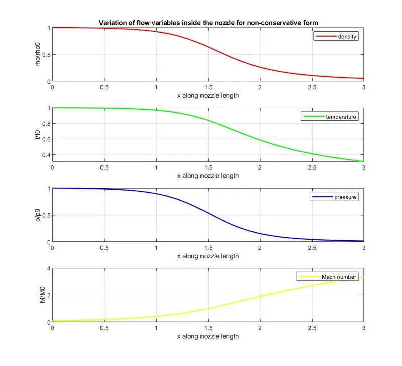
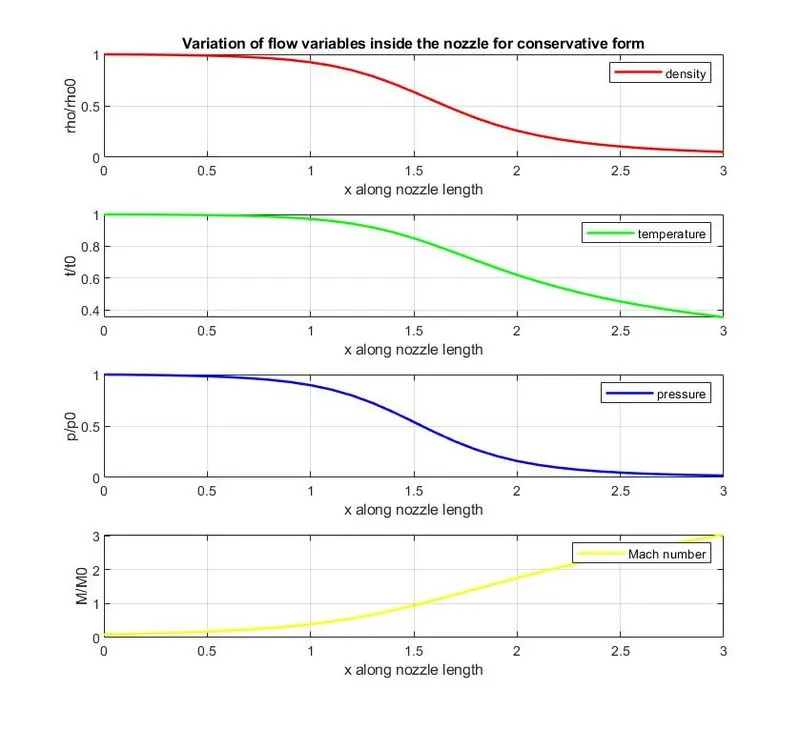
Density, temperature, pressure all decrease downstream the nozzle, whereas the Mach number increases as the flow accelerates beyond sonic velocity and reaches super sonic conditions at the outlet.
Conservative
2)Time-wise variation
Non-conservative
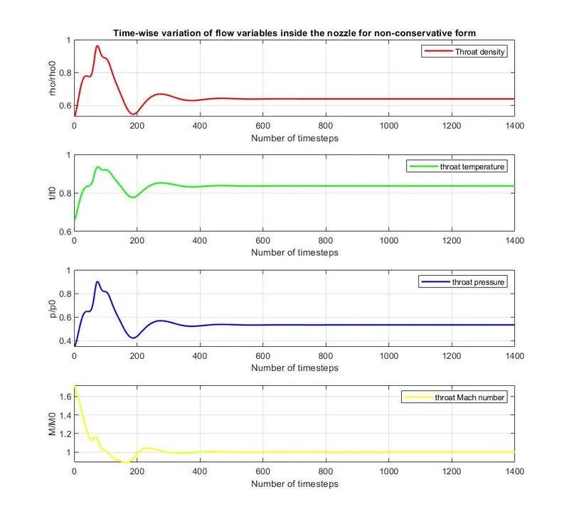
As seen from the graphs, the changes in the primitive variables are largest at early timesteps, after which the steady state is obtained with the graphs being asymptotic. Initially the field variables have greater potential for change, like the 'rubber band effect'. The time derivatives are large initially and hence affect changes in variables. As the solution progresses, the change in time derivatives decreases and the primitive variables attain a steady state.
Conservative
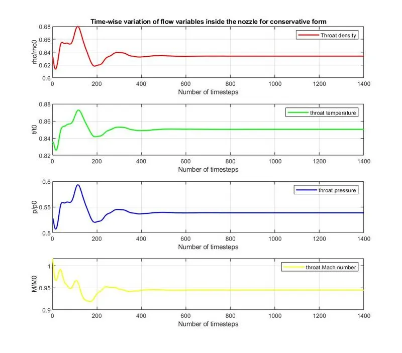
3)Variation of mass flow rate inside the nozzle at different time-steps.
Non-conservative
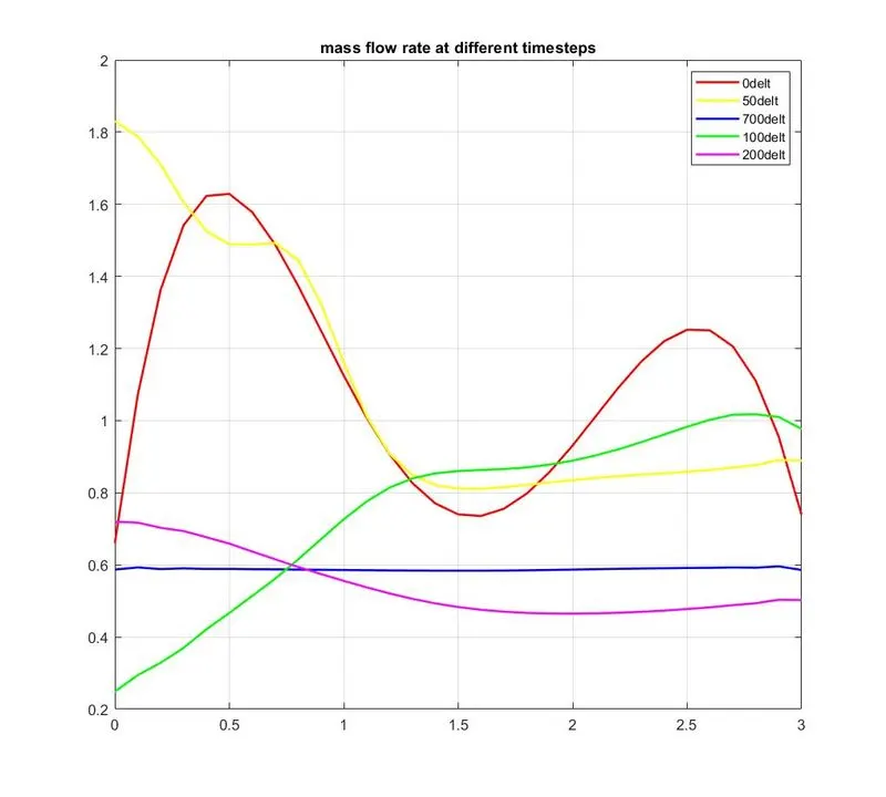
Initially, at zero time step, the flow rate(rho*v*a) has somewhat sinusoidal appearance(red curve), as we assumed initlal parabolic variation for area combined with rho and v. After 200delt, the flow rate starts to settle down (magenta). At 700delt it is constant and equal to analytical value of 0.579.
Conservative
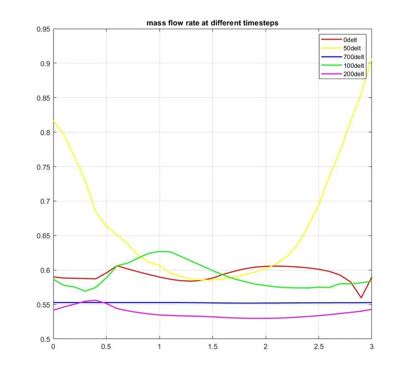
4) Normalized flow rate distribution of both non-conservative and conservative.
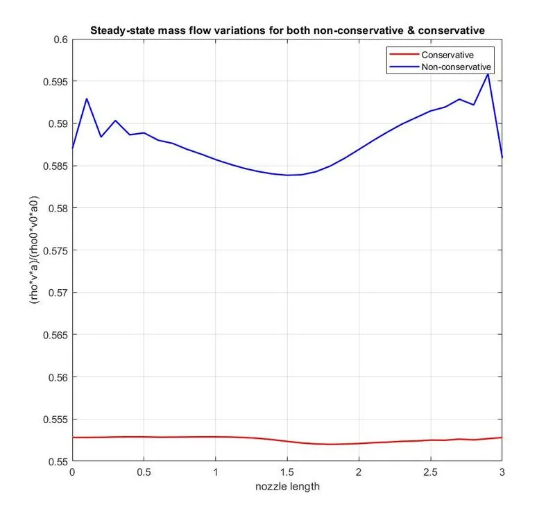
The steady state distribution of mass flow rate shows that the conservative form is much closer to being a constant than non-conservative. The non-conservative has sizeable variations at both inflow and outflow. The conservative form is closer to the analytical value.
5)Grid-independence test.
| rho*/rho0 | t*/t0 | p*/p0 | M | |
| Exact analytical solution | 0.634 | 0.833 | 0.528 | 1 |
| Non-conservation form, numerical results(31 points) | 0.6386 | 0.8364 | 0.5342 | 0.9993 |
| Non-conservation form, numerical results(61 points) | 0.6375 | 0.8353 | 0.5326 | 0.9997 |
| Conservation form, numerical results(31 points) | 0.6338 | 0.8503 | 0.5389 | 0.9448 |
| Conservation form, numerical results(61 points) | 0.6343 | 0.8522 | 0.5406 | 0.9382 |
The results show for the grid independence test show that the primitive variables are slightly closer to the exact values and the change in grid points does not affect the solution very much.
The non-conservative, 31 points results are much closer to the exact analytical values than conservative, 61 points.