Week 3.5 - Deriving 4th order approximation of a 2nd order derivative using Taylor Table method

Second order derivatives appear in the Navier Stokes equations for viscous flows. To discretize second-order derivatives, the Taylor series can be used to determine the finite difference expressions.

1) Central differencing

In central differencing scheme, points left and to the right of the concerned point in the numerical stencil are used to evaluate the expression, i.e. points ranging from 'i-k' to 'i+k' are considered. For this case since a fourth order accuracy is required, we shall consider points from 'i-2' to 'i+2'.

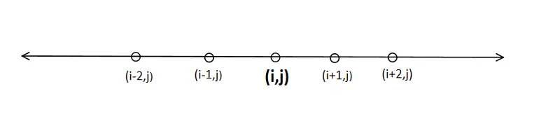
Number of nodes in the stencil N = 5

Order of derivative Q = 2

`(del^2f)/(delx^2)` = a*f(i-2)+b*f(i-1)+c*f(i)+d*f(i+1)+e*f(i+2)

Expanding the terms by Taylor series and comparing the coefficients, we represent it in a table format.

	f(x)	(`Deltax`)*f'(x)	(`Deltax`)^2*f''(x)	(`Deltax`)^3*f'''(x)	(`Deltax`)^4*f''''(x)
a*f(i-2)	a	-2*a	2*a	-8*a/6	16*a/24
b*f(i-1)	b	-b	b/2	-b/6	b/24
c*f(i)	c	0	0	0	0
d*f(i+1)	d	d	d/2	d/6	d/24
e*f(i+2)	e	2*e	2*e	8*e/6	16*e/24
Summation of terms `(del^2f)/(delx^2)`	0	0	1	0	0

From this we get a system of linear equations which can be solved using matrices in Matlab to get the values for the coefficients.

`(del^2f)/(delx^2)` = (-f(i+2) +16*f(i+1) -30*f(i) +16*f(i-1)-f(i-2))/12*(`Deltax`)^2

coefficients are,

i-2	i-1	i	i+1	i+2
a	b	c	d	e
-1/12	4/3	-5/2	4/3	-1/12

The order of accuracy P= N - Q +1 = 5-2+1 = 4

The Central difference scheme is fourth order accurate.

2)Skewed right-sided difference

The right-sided difference uses information from the right of the grid- point(i,j). Consider points from i to i+5.

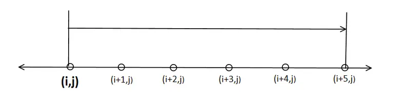
`(d^2x)/dx^2 = a*f(i) + b*f(i+1) + c*f(i+2) + d*f(i+3) + e*f(i+4) + f*f(i+5)`

Number of nodes in the stencil N = 6

Order of derivative Q = 2

	f(x)	(`Deltax`)*f'(x)	(`Deltax`)^2*f''(x)	(`Deltax`)^3*f'''(x)	(`Deltax`)^4*f''''(x)	(`Deltax`)^5*f'''''(x)
a*f(i)	a	0	0	0	0	0
b*f(i+1)	b	b	b/2	b/6	b/24	b/120
c*f(i+2)	c	2*c	2*c	8*c/6	16*c/24	4*c/15
d*f(i+3)	d	3*d	9*d/2	9*d/2	27*d/8	81*d/40
e*f(i+4)	e	4*e	8*e	32*e/3	32*e/3	128*e/15
f*f(i+5)	f	5*f	25*f/2	125*f/6	625*f/24	625*f/24
Summation	0	0	1	0	0	0

The coefficients turn out to be,

i	i+1	i+2	i+3	i+4	i+5
a	b	c	d	e	f
15/4	-77/6	107/6	-13	61/12	-5/6

The order of accuracy P = N-Q = 6-2 = 4

The Skewed right-sided scheme is fourth order accurate.

3) Skewed left-sided

The right-sided difference uses information from the left of the grid-point(i,j). Consider points from i to i-5.

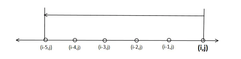
`(d^2x)/dx^2 = a*f(i) + b*f(i-1) + c*f(i-2) + d*f(i-3) + e*f(i-4) + f*f(i-5)`

Number of nodes in the stencil N = 6

Order of derivative Q = 2

	f(x)	(`Deltax`)*f'(x)	(`Deltax`)^2*f''(x)	(`Deltax`)^3*f'''(x)	(`Deltax`)^4*f''''(x)	(`Deltax`)^5*f'''''(x)
a*f(i)	a	0	0	0	0	0
b*f(i-1)	b	-b	b/2	-b/6	b/24	-b/120
c*f(i-2)	c	-2*c	2*c	-8*c/6	16*c/24	-4*c/15
d*f(i-3)	d	-3*d	9*d/2	-9*d/2	27*d/8	-81*d/40
e*f(i-4)	e	-4*e	8*e	-32*e/3	32*e/3	-128*e/15
f*f(i-5)	f	-5*f	25*f/2	-125*f/6	625*f/24	-625*f/24
Summation	0	0	1	0	0	0

The coefficients are,

i	i-1	i-2	i-3	i-4	i-5
a	b	c	d	e	f
15/4	-77/6	107/6	-13	61/12	-5/6

The order of accuracy P = N-Q = 6-2 = 4

The Skewed left-sided scheme is fourth order accurate.

MATLAB code for 2nd order derivative of exp(x)*cos(x)

Function for central differencing scheme

function error_cds = cds_ddx(x,dx)
%central differencing scheme
A = [1 1 1 1 1; -2 -1 0 1 2; 2 1/2 0 1/2 2; -8/6 -1/6 0 1/6 8/6; 16/24 1/24 0 1/24 16/24];
B = [0; 0; 1; 0; 0];
coeffcds = (inv(A))*B;
varcds = [exp(x-2*dx)*cos(x-2*dx) exp(x-dx)*cos(x-dx) exp(x)*cos(x) exp(x+dx)*cos(x+dx) exp(x+2*dx)*cos(x+2*dx)]; 
secondcds = varcds*coeffcds/dx^2;
second_ddx = -2*exp(x)*sin(x);
error_cds = abs(secondcds - second_ddx);
end

Function for skewed right-sided scheme

function error_fds = fds_ddx(x,dx)
%skewed right-sided
A1 = [1 1 1 1 1 1;0 1 2 3 4 5;0 1/2 2 9/2 8 25/2;0 1/6 8/6 9/2 32/3 125/6;0 1/24 16/24 27/8 32/3 625/24;0 1/120 4/15 81/40 128/15 625/24];
B1 = [0; 0; 1; 0; 0; 0];
coefffds = (inv(A1))*B1;
varfds = [exp(x)*cos(x) exp(x+dx)*cos(x+dx) exp(x+2*dx)*cos(x+2*dx) exp(x+3*dx)*cos(x+3*dx) exp(x+4*dx)*cos(x+4*dx) exp(x+5*dx)*cos(x+5*dx)];
secondfds = varfds*coefffds/dx^2;
second_ddx = -2*exp(x)*sin(x);
error_fds = abs(secondfds-second_ddx);
end

Function for skewed left-sided scheme

function error_rds  = rds_ddx(x,dx)
%skewed left-sided
A2 = [1 1 1 1 1 1;0 -1 -2 -3 -4 -5;0 1/2 2 9/2 8 25/2;0 -1/6 -8/6 -9/2 -32/3 -125/6;0 1/24 16/24 27/8 32/3 625/24;0 -1/120 -4/15 -81/40 -128/15 -625/24];
B2 = [0; 0; 1; 0; 0;0];
coeffrds = (inv(A2))*B2;
varrds = [exp(x)*cos(x) exp(x-dx)*cos(x-dx) exp(x-2*dx)*cos(x-2*dx) exp(x-3*dx)*cos(x-3*dx) exp(x-4*dx)*cos(x-4*dx) exp(x-5*dx)*cos(x-5*dx)];
secondrds = varrds*coeffrds/dx^2;
second_ddx = -2*exp(x)*sin(x);
error_rds = abs(secondrds-second_ddx);
end

These functions take inputs from the Taylor tables for the respective schemes and output a coefficient matrix. The coefficient matrix and the function/variables matrix together form the expression for the second-order derivative.

It is then compared with the analytical derivative by defining a error variable. All three of the error variables are then compared in the main program below.

clear all
close all
clc

x = pi/2;
dx = linspace(pi/4,pi/4000,20);

for i = 1:length(dx)
   central_error(i) = cds_ddx(x,dx(i));   
   forward_error(i) = fds_ddx(x,dx(i));
   rearward_error(i) = rds_ddx(x,dx(i));
end

loglog(dx,central_error,'r')
hold on;
loglog(dx,forward_error,'g')
hold on;
loglog(dx,rearward_error,'b')
xlabel('dx')
ylabel('error')
title('plot of dx v/s error for central, forward, rearward')
legend('CentralDS','ForwardDS','RearwardDS')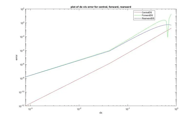

A] The central differencing scheme is more accurate as compared to the skewed right and left sided schemes.

The slope of the error v/s dx graph is constant for central differencing scheme, whereas it changes for both right and left schemes at a certain value of 'dx'.

B] The one-sided or skewed schemes are generally useful where information is available only on one side of the domain. For eg, in viscous flow calculations, the shear stress at the wall due to the flow over the wall. The gradient of velocity at the wall has to be calculated from points only on one side of the wall.

The Central differencing scheme employs equal number of points from either side of the point of interest. It cannot be used at a boundary. Moreover, if the function of interest is a oscillatory function, the central differencing scheme will generate a zero derivative.