Week 3 - External flow simulation over an Ahmed body.

INTRODUCTION

Ahmed body & its importance

The flow past an automobile (cars, buses, trucks) under normal operating conditions is primarily turbulent. It has general characteristics of flow-separation, recirculation regions, wake flow, trailing vortices and interaction of boundary layer with vehicle.

These phenomena influence the principal features such as shape of vehicle, aerodynamic drag, fuel consumption, noise production and road handling. The understanding of these has been gained through wind tunnel testing. However, CFD has enabled to determine the drag and lift coefficients without using a wind tunnel. A road-vehicle is essentially a bluff-body with very close ground proximity. As typical for a bluff-body, the major contribution to drag experienced by a road vehicle is pressure drag.

To test turbulence models for complex geometries, a simplified car model known as Ahmed body is used as a benchmark. It is a generic model of a passenger car made up of a round front part, a slant plane at the rear to study the separation phenomenon and to study the coefficient of drag, a main body of rectangular shape connecting the front and rear slant plane.

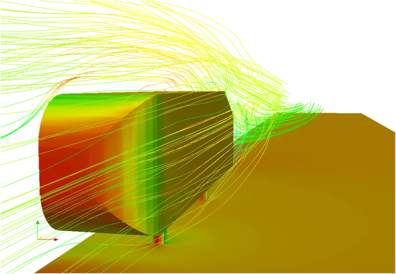
Current vehicles involve complex geometries due to the accessories and devices that are involved which make the validation and analysis task unaffordable. The Ahmed body is a simple model which retains the essential flow features, specially the vortex wake flow.

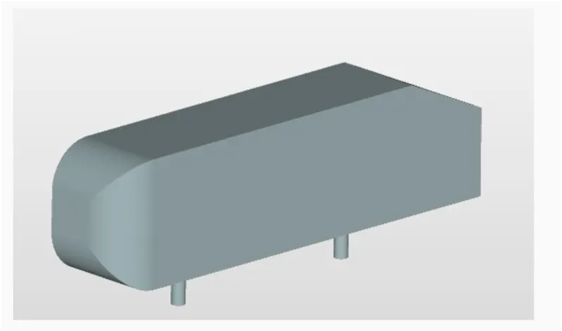
The objectives for this project are

1. To analyze air flow over the Ahmed body and determine the drag coefficient using CFD (Ansys Fluent).
2. To perform simulation for a half-body using symmetry boundary condition.
3. To implement turbulence model (k-ε, RANS) with suitable wall functions, based on calculations of y+.
4. To create a refined mesh for the setup this involves a region of influence around the Ahmed body that includes the wake region. Also a fluid domain which encloses the Ahmed body & the region of influence.
5. Analyze the wake pattern (recirculation, vortices) at the rear part of the model.
6. To perform grid-independency test and compare drag & lift coefficients for each case.

GEOMETRY OF AHMED BODY

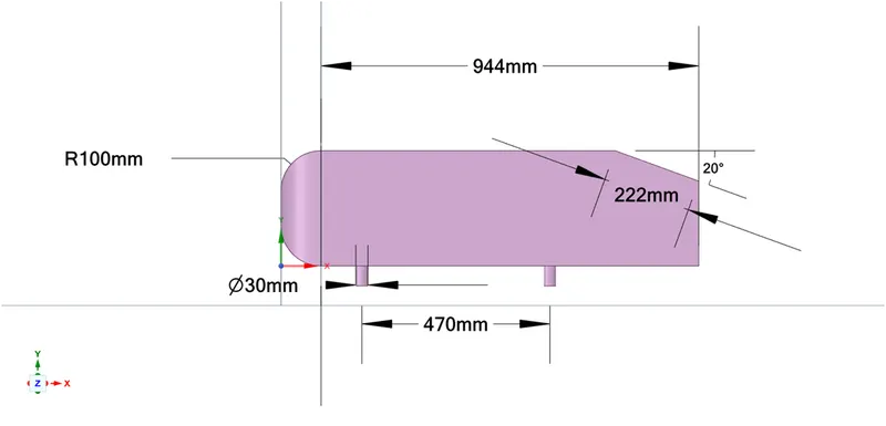
The geometry of the Ahmed body is imported in SpaceClaim. It has a rounded front part with a rectangular nose. At the rear, there is a slant plane of 20°. The model has a ground clearance with four cylindrical supports simulating the wheels.

Side View

Front View

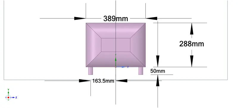
The dimensions of the Ahmed body are as follows

Length	944 mm
Height	288 mm
Width	389 mm
Ground clearance	50 mm
Slant plane angle	20°
Slant plane length	222 mm
Front radius	100 mm

MODELLING & MESH REQUIREMENTS

The flow over Ahmed body is characterized by boundary layer, vortices, flow separation, recirculation.

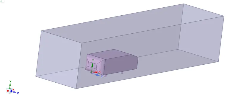
To accurately simulate these phenomena, the mesh needs to be fine and refined in the regions where these phenomena dominate. For this setup, the flow domain is divided into three regions.

1. Ahmed body
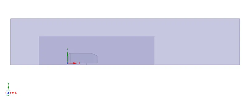
2. Region of influence: - Includes the wake region.
3. Fluid domain which acts as a wind tunnel

Since the flow is external over the Ahmed body, there is no need for meshing inside the body. For this purpose, the ‘Enclosure’ option in SpaceClaim is used. This creates a cubical enclosure around the model and retains the shape of the model.

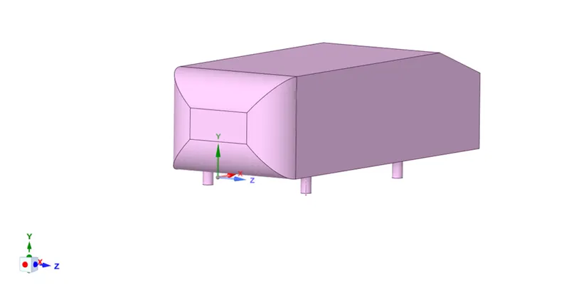
Ahmed body model in SpaceClaim

Region of influence

Fluid domain around the Ahmed body

The shape retained by the enclosure acts as the model for the flow simulation and the actual model is then suppressed for physics.

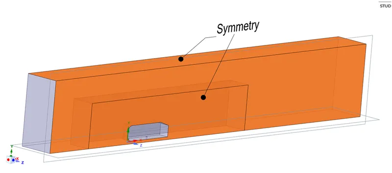
The flow is symmetric past the model & hence only half of the body can be simulated by applying symmetry boundary condition along the split plane. This is done using the ‘Split Body’ option in SpaceClaim.

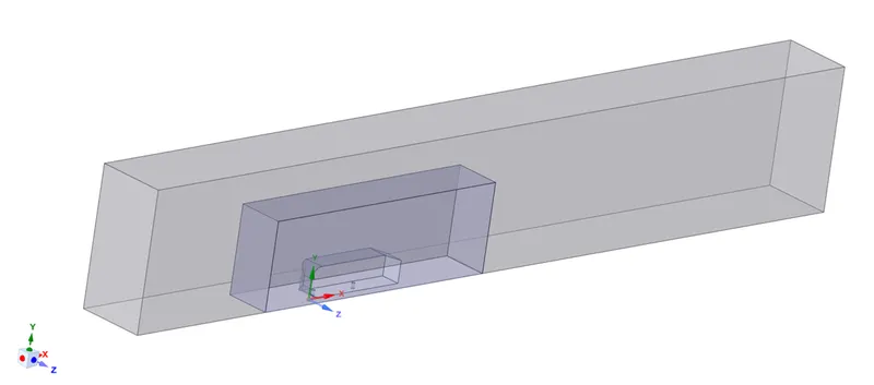
Flow domain split along the YZ plane.

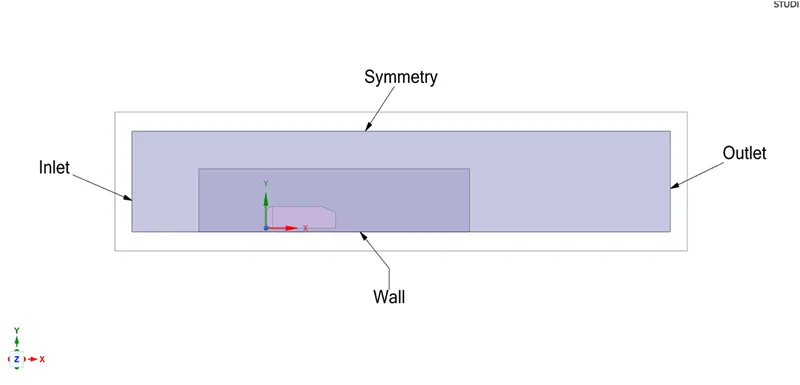
The boundaries are defined as follows

1. Inlet
2. Outlet
3. Symmetry ( Fluid domain planes along Y & Z axes and the split plane)
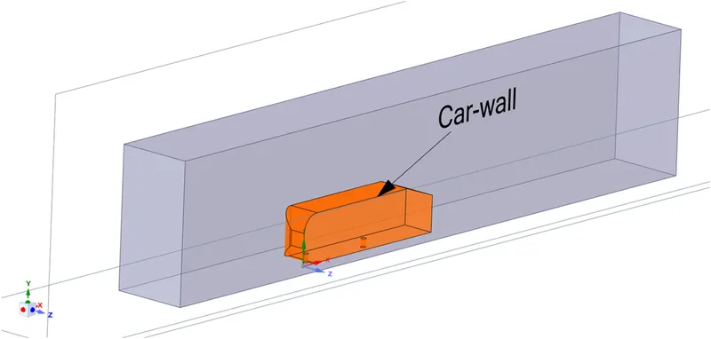
4. Wall (Ahmed body & the plane on which it rests).

Ahmed Body wall

Symmetry along the split plane

MESH

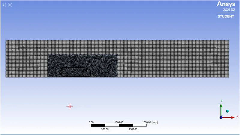
The generated mesh for the model is as follows

Mesh type & element size

• Fluid domain: Hexahedral structured, 50 mm (global setting).
• Region of influence: Body sizing, 25 mm.
• Car wall: Inflation layers 6, 39.71 mm.
• Cylindrical supports: Face sizing, 10 mm

As seen from above the mesh is refined in the region of influence. Around the model there is an inflation layer made up of 6 layers with a growth rate of 1.2 having total thickness of 39.71 mm. The fluid domain has a structured mesh of hexahedral element type. Since the type of mesh between the region of influence and fluid domain is different, the meshes overlap one another. This happens due to the interference between the two regions. This is overcome by using the interference option in SpaceClaim which makes the transition from one region to another smoothly.

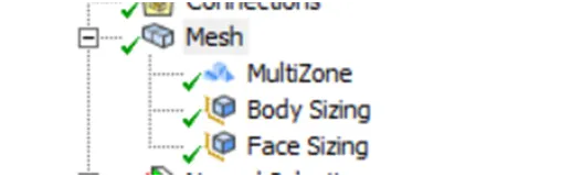
• MultiZone: - Generates a pure hexahedral mesh without slicing the region. In this case, the fluid domain.
• Body Sizing: - Defines an element size for the region of influence body.
• Face sizing: - Defines an element size for the cylindrical supports.

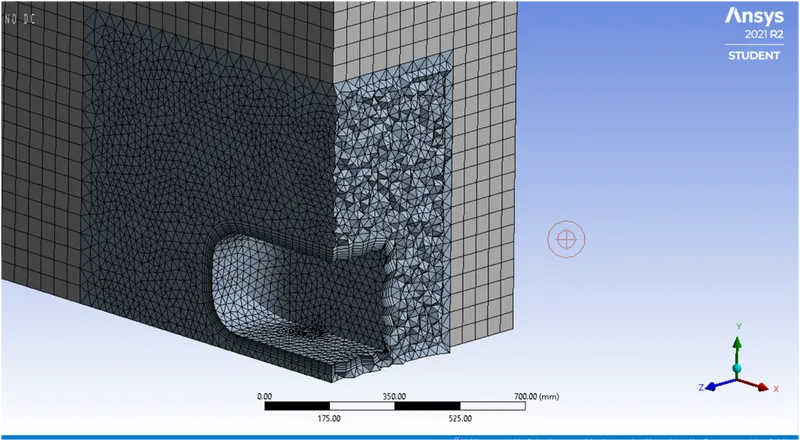
Y+

To determine the thickness of inflation layers, y+ is used. For turbulent flow past a surface, the near-wall region plays an important role as the velocity gradients are the most in this region. The velocity gradients affect the shear stress and in turn the flow. The region near the wall for turbulent flow is divided into different regions based on the velocity profile and the fluid-flow behaviour.

• The viscous-sublayer: Viscous effects are significant, velocity profile is linear, flow is streamlined
• Buffer layer: Turbulent effects are becoming significant
• Overlap layer: Turbulent effects are much more significant, logarithmic velocity profile.

Y+ is a nondimensional distance from the wall. It is defined as,

`y+ = y*u^**/nu`

Where

• y is the actual distance from the wall in m.
• `u^**` is the friction velocity defined as `u^** = sqrt(tau_w/rho)`in m/s.
• `nu` is the kinematic viscosity in m^2/s.

Similar to y+, there is a nondimensional velocity u+ defined as

`u+ = u/u^**`

Y+ is plotted against u+ based on experimental values and the results are,

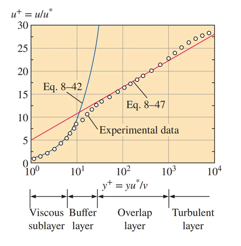
Source: - Fluid Mehanics Fundamentals & applications, Cengel & Cimbala, 4th edition.

For the viscous sublayer the law for velocity profile is

y+ = u+

While the overlap layer follows a logarithmic profile according to the equation

`u+ = 2.5*log(y+) + 5`

Need for y+ is to distinguish between the different regions near the wall or viscous regions.

In viscous sublayer y+ < 5

Buffer layer 5 < y+< 30

Overlap layer 30 < y+ < 500

To determine the cell size near the wall there are two approaches

1. Full resolution in the near-wall region: y+ < 1
2. Using wall functions to resolve near-wall region: 30 < y+<300

A full resolution of mesh in the near-wall region would generate more element cells and hence require more computational time & resources.

Using wall functions to resolve near-wall region is the appropriate choice for this case.

For y+ = 200, the calculation of the inflation layer thickness is

• Free stream velocity `u_infty`= 25 m/s
• Density of air ρ = 1.225 kg/m^3
• Viscosity µ = 1.7894e-05 kg/(m-s)
• Length of car l = 0.94 m
• Reynolds number `Re = rho*u_infty*l/mu`= 1,711,467.531
• Skin friction coefficient `C_f = 0.0576*(Re)^(1/5)` = 3.264e-03
• Wall shear stress `tau_w = 1/2*C_f*rho*(u_infty)^2` = 0.624 Pa
• Friction velocity `u^** = sqrt(tau_w/rho)` = 0.71414 m/s

y+ = 200 = `y*u^**/nu`

Which gives y = 4.09 mm. This is the height or thickness of the first layer adjacent to the wall. Based on this value a total of 6 layers are added near the wall with a growth rate of 1.2. The calculation of total thickness is done below.

y+ = 200	layer no	thickness in mm
	1	4
	2	4.8
	3	5.76
	4	6.912
	5	8.2944
	6	9.95328
	Total thickness	39.71968

SOLVER REQUIREMENTS

The k-epsilon model for turbulence is employed which in addition to the fluid continuity and momentum, solves equations for the turbulent kinetic energy k and the rate of dissipation of turbulent kinetic energy ( epsilon). These are based on Reynolds Averaged Navier Stokes (RANS) equations.

`(delrho)/(delt) + grad*(rho*vecV) = 0`

`rho*(DvecV)/(Dt) = -vecgradP + rho*vecg + mu(grad^2vecV)`

K-epsilon is a high Reynolds number model which is most suitable for fully developed turbulent flows away from the wall. For this model, wall functions are used to bridge the viscosity affected region between the wall and the turbulent region.

For this case, Scalable wall function is used.

Solver: Pressure-based

Time: Steady

Pressure-velocity coupling: SIMPLE

Initialization: Hybrid

POST-PROCESSING & RESULTS

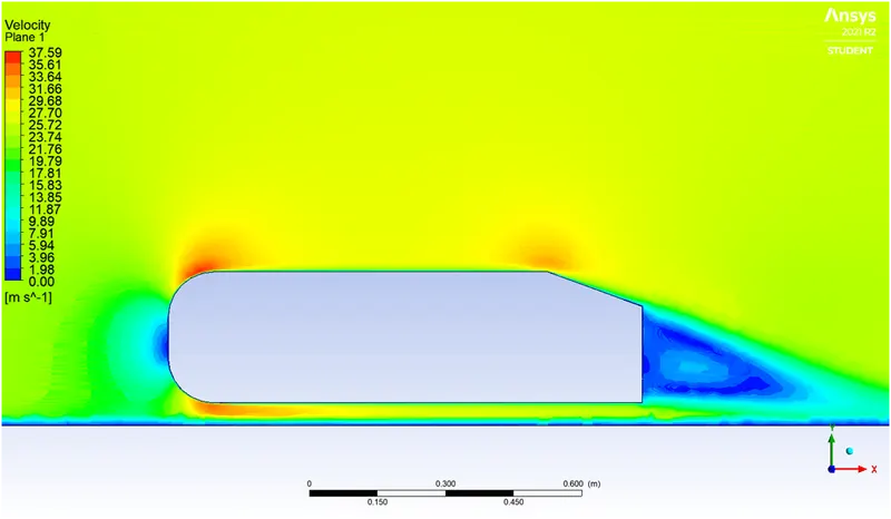
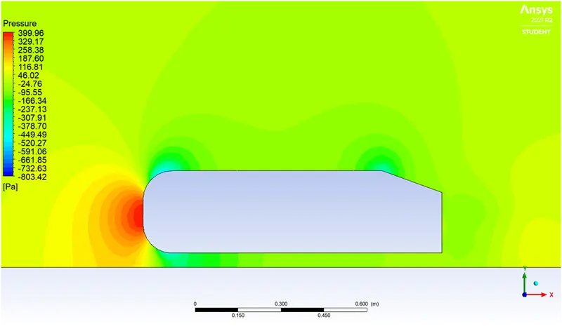
The simulation for a refined setup was run for a free stream velocity of 25 m/s and the contour plots of velocity and pressure are plotted in CFD-post.

Velocity contour

Pressure contour

INFERENCES

• At the nose of the body in front, the fluid flow comes to a stop at the stagnation point. The velocity is zero at this point. The stagnation pressure is equal to the dynamic pressure plus the atmospheric pressure and is maximum at this point.
• In the rear part of the body the pressure is negative. This happens due to the boundary layer separation. The streamlines close to the body are not able to follow the shape of the body. The dividing streamline passes through the separation point. Above the dividing streamline, the fluid continues downstream. This leads to a region of low pressure in the immediate rear part of the body. Some streamlines are caught in this region and begin recirculating.
• Along the wall of the body the boundary layer develops due to the no-slip condition. This boundary layer separates at the slant plane in the rear part of the body.

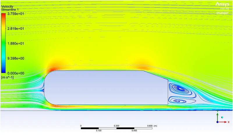
• The point of separation is the point at which the boundary layer separates from the surface. Boundary layer separation occurs where the rear portion experiences an adverse pressure gradient and a decelerating flow.
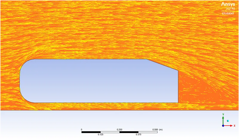
• In the streamline plot, two closed streamlines are formed in the rear end of the body. These represent regions of recirculating flow. One streamline from lower part of the body & one from the upper part of the body are caught in this region. There is reverse flow in these regions and a strong y-component of velocity present in this region beyond the separation point.
• The boundary layer equations are not valid in this region.
• As compared to laminar boundary layers, the turbulent boundary layers are more resistant to separation. This is because the velocity profiles in case of turbulent flow are much more developed and close to the mean flow velocity.

Vector plot showing reversed flow

RESULTS

Drag coefficient `C_d`	Lift coefficient `C_l`
0.33262	0.28605

GRID INDEPENDENCY TEST

Fluid domain mesh size: - 50 mm.

Region of influence mesh size in mm	Number of cells	Drag-coefficient	Lift-coefficient
50	124212	0.39113	0.32743
35	233933	0.36052	0.31891
30	331672	0.34009	0.28507
25	510861	0.33262	0.28605

As we decrease the mesh size,

• The changes in the drag & lift coefficients are small.
• The number of elements/cells increases, which increases computational time.
• In addition to that, the limit for the Ansys student version is 512k cells.
• Hence, at the mesh size of 25 mm, grid independency is achieved.
• At 25 mm, the value of drag coefficient is closest to the theoretical value of 0.33.