Week 5 - Curve fitting

AIM- To write a PYTHON code that performs curve-fitting on the relationship between cp and Temperature and finding the PERFECT FIT for the following.

THEORY- Curve fitting is the process of constructing a curve, or mathematical functions, which possess the closest proximity to the real series of data. By curve fitting, we can mathematically construct the functional relationship between the observed dataset and parameter values, etc.

The accuracy of the curve fit can be improved by increasing the degree of the polynomial.

So, a 'Best fit' can be obtained by increasing the degree of the polynomial.

PERFECT FIT: The perfect fit is achieved when the geometric distances from the given points to the fitting curve are zero . This means that the curve fits perfectly on the points.

To get a perfect fit we can increase the order of the polynomials, this method increases the accuracy and reduces errors.

BEST FIT: The best fit is achieved when the geometric distances from the given points to the fitting curve are minimized, in the least-squares sense. Finding the best fit reduces to the minimization of the objective function where denotes the fitting curve.

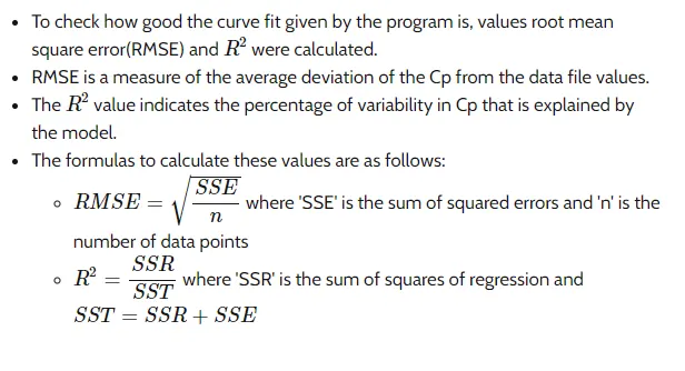
Upon finding a curve that satisfies the data points there are 4 quantities that help us measure the goodness of fit criteria or how well the equation is representing the data points. There are,

The sum of squares due to error (SSE)

R-square

R-squareAdjusted

R-square-root mean squared error (RMSE)

What is the difference between a PERFECT FIT and BEST FIT

Best fit simply means that the differences between the actual measured Y values and the Y values predicted by the model equation are minimized. It does not mean a "perfect" fit; in most cases, a least-squares best fit does not go through all the points in the data set.

PERFECT FIT refers to the goodness of FIT, it is determined by the four methods mentioned above.

PYTHON CODE

#curve_fit using Python

#Importing the modules required 
import math
import matplotlib.pyplot as plt 
import numpy as np
from scipy.optimize import curve_fit

def fn_linear(t,a,b):                                        #linear function to provide a linear Fit
	return a*t+b
	
def fn_cubic(t,a,b,c,d):                                     #cubic function to provide a cubic Fit                
	return a*pow(t,3)+b*pow(t,2)+c*t+d
	
def read_file():									         #reading data file
	temperature=[]
	cp=[]
	for line in open('data','r'): #(data,r)-->r here stands for read
		values = line.split(',') #splitting the data into two
		temperature.append(float(values[0])) # First value is temperature 
		cp.append(float(values[1])) #Second value is cp
		
	return [temperature,cp] #The function will return a array of temperature and cp


temperature,cp = read_file() #Read file function will read the data file

popt, pcov =curve_fit (fn_linear,temperature,cp)              #Curve Fit for linear
fit_cp_linear = fn_linear(np.array(temperature),*popt)

popt, pcov =curve_fit (fn_cubic,temperature,cp)				  #Curve Fit for cubic
fit_cp_cubic = fn_cubic(np.array(temperature),*popt)

plt.plot (temperature,cp,'r')								  #Plot for Linear
plt.plot (temperature,fit_cp_linear,'b')
plt.show()

plt.plot (temperature,cp,'r')								  #Plot for Cubic
plt.plot (temperature,fit_cp_cubic,'b')
plt.show()
#Emperical Calculation of R^2,SSE ,RMSE
MEAN = np.mean(cp)

ERROR1 = np.array (cp) - np.array (fit_cp_linear)                  #Calculation for linear
ERROR_SQ1=np.square(ERROR1)
SSE1 = sum (ERROR_SQ1)
SSR1 = [x - MEAN for x in fit_cp_linear]
SSR_SQ1 =np.square(SSR1)
SSRR1 = sum (SSR_SQ1)
R_SQ1 = 100*SSRR1/(SSRR1+SSE1)
RMSE1 = pow((SSE1/3200),0.5)
print (R_SQ1,'...R_SQ linear')
print (RMSE1,'...RMSE linear')
print ('------------------------------------')

ERROR2 = np.array (cp) - np.array (fit_cp_cubic)                  #calculation for cubic
ERROR_SQ2=np.square(ERROR2)
SSE2 = sum (ERROR_SQ2)
SSR2 = [x - MEAN for x in fit_cp_cubic]
SSR_SQ2 =np.square(SSR2)
SSRR2 = sum (SSR_SQ2)
R_SQ2 = 100*SSRR2/(SSRR2+SSE2)
RMSE2 = pow((SSE2/3200),0.5)
print (R_SQ2,'...R_SQ cubic')
print (RMSE2,'...RMSE cubic')
print ('------------------------------------')

RESULTS

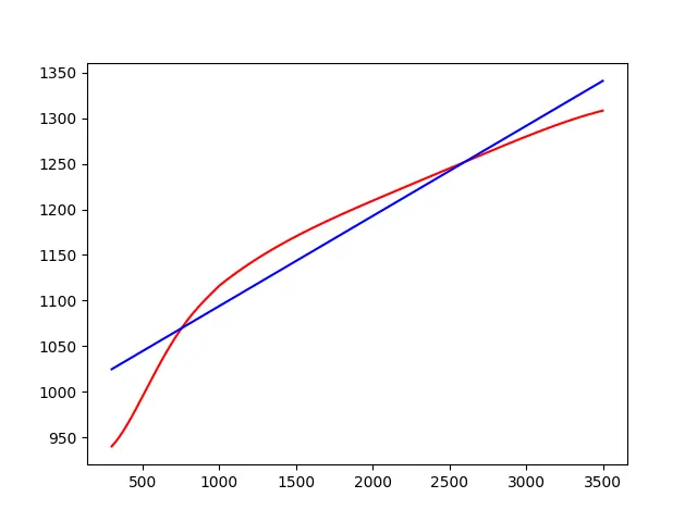
-->Linear

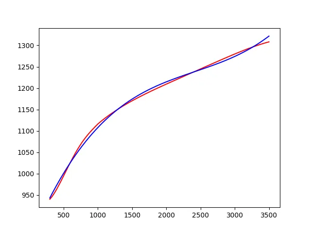
--->Cubic

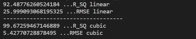
-->Emperical Calculation

Observations

• Three curve fits (blue curve) were plotted along with the original curve (red curve) for comparison as shown below. It was observed that the higher the degree of the polynomial used for curve fit better the accuracy of the curve was. Alternatively, lower degree polynomials can be split into multiple parts to better fit the curve. In the three curves plotted below best fit was observed for the linear curve split into multiple(8 in this case) parts.
• The values of RMSE and R square were calculated for each of the curves as shown below. It was observed that the value of RMSE was lowest for the cubic curve and the linear curve had the highest RMSE value. The R square value was found to be the highest for the cubic curve.