Week 2 Air standard Cycle

AIM:
To generate the PV diagram and to determine the thermal efficiency of the engine.

The programming language used is Python

THEORY:

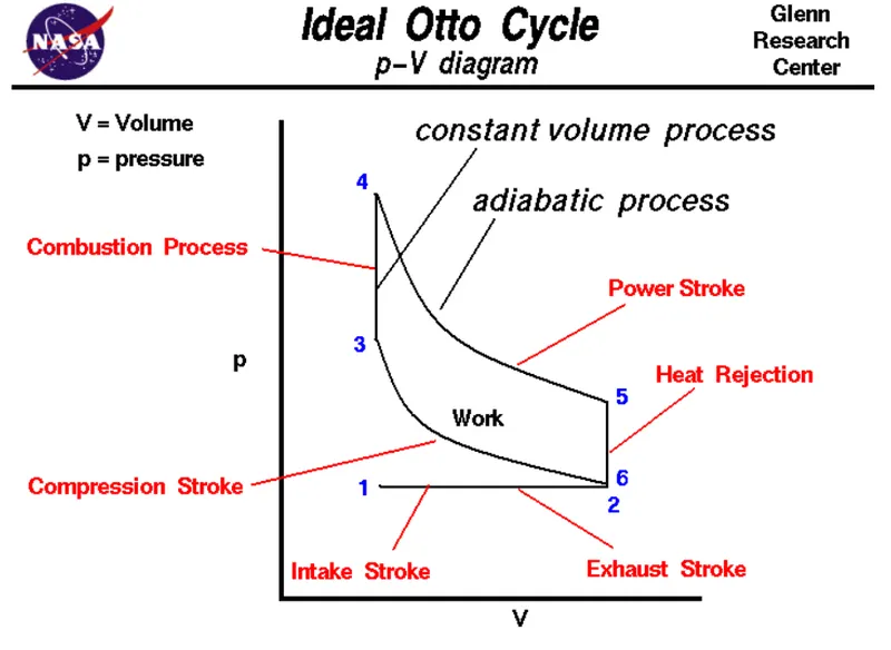
Otto Cycle is an idealized thermodynamic cycle that describes the working of a spark-ignition engine. The cycle consists of 4 processes as illustrated in the figure below:

it consists of 4 strokes namely:

1.Suction Stroke(1-2): The charge is compressed isentropically to a smaller volume and hence the pressure and temperature increase to p2,t2 from p1,t1.

2.Compression Stroke(2-3): In this stage, the heat is added at constant volume hence the pressure and temperature increase to p3,t3

3.Expansion Stroke(3-4): The charge is expanded isentropically hence the pressure and temperature reduces to p4,t4

4. Exhaust stroke(4-1): The heat is removed keeping the volume constant, hence reduces the pressure and temperature to p1,t1.

Engine kinematics is used to plot changing values of volume as the piston is moving from Top Dead Centre(TDC) to Bottom Dead Centre(BDC). Hence it is a function of bore, stroke, length of connecting rod and crank angle

Various geometric parameters of the engine are used to calculate Clearance volume(V_c), Swept volume(V_s) and other coordinates of properties they are:

1.Bore(bore):Diameter of cylinder

2.Stroke(stroke): Length that the piston travels from TDC to BDC

3.Length of connecting rod(con_rod)

4.Compression ratio(cr): Degree to which the fuel mixture is compressed

5.Crankpin radius(a)=stroke/2

6.A constant, R=con_rod/a

The isentropic curve is plotted by finding out the volume trace which is given by :

PYTHON CODE:

• The Programme is divided into two parts
• The first part contains the program for otto cycle and the second part in which the function for Trace volume is defined
• The function is being imported into the main program using[ from(file name) import(space)*]
• The engine parameters such as engine bore dia, compression ratio, stroke length, and connecting rod length are given as input.
• Initial conditions such as temperature and pressure at first state point and temperature at state point 3 are given and constant gamma is specified.
• Using the above input volume is calculated.
• State 2, state 3 and state 4 variables are calculated, using conditions and formulas.
• To visualize the actual variation of volume with pressure between state 1 to 2 and state 3 to 4, Functions 'engine_kinematics' is created.In function start_angle, end_angle are the crank angles( it defines the piston position in the cylinder and hence also defines volume).
• volume relation

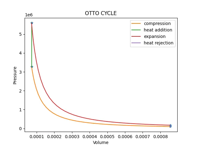
• State points, process path are defined plotted using 'plt.plot()'
• Thermal efficiency calculated using relation thermal efficiency = 1-(1/cr^(gamma-1))
  

PART-1

from engine_Kinematics import *
import math
import matplotlib.pyplot as plt
#Otto cycle simulator
#Inputs
p1 = 101325 
t1 = 500
gamma = 1.4
t3 = 2300
#Geometric parameters of the Engine
bore = 0.1
stroke = 0.1
con_rod = 0.15
cr = 8
#Volume computation
V_s= (math.pi/4)*pow(bore,2)*stroke
V_c= V_s/(cr-1)
V1= V_s+V_c
#State point 2
V2 = V_c
#p2v2^gamma = p1v1^gamma
p2 = p1*pow(V1,gamma)/pow(V2,gamma)
#p2v2/t2=p1v1/t1|rhs=p1v1/t1|p2v2/t2=rhs|t2=p2v2/rhs
rhs=p1*V1/t1
t2=p2*V2/rhs
V_compression = engine_Kinematics(bore,stroke,con_rod,cr,180,0)
constant = p1*pow(V1,gamma)
P_compression=[]
for v in V_compression:
    P_compression.append(constant/pow(v,gamma))
#State point 3
V3= V2
#p3v3/t3 = p2v2/t2|rhs=p2v2/t2|p3=rhs*t3/v3
rhs=p2*V2/t2
p3=rhs*t3/V3
V4 = V1
#p4v4^gamma = p3v3^gamma
p4 = p3*pow(V3,gamma)/pow(V4,gamma)
#p4v4/t4=rhs
t4=p4*V4/rhs
V_expansion =engine_Kinematics(bore,stroke,con_rod,cr,0,180)
constant2 = p3*pow(V3,gamma)
P_expansion = []
for v in V_expansion:
    P_expansion.append(constant2/pow(v,gamma))
#State point 4

'''Thermal efficiency nth of the otto cycle(engine)
efficiency = fraction of heat converted to work
nth = W/Q
nth = 1 - (QL/QH)'''

NTH = 1 - 1/(pow(cr,(gamma-1)))
print('Thermal Efficiency of the Engine is:' +str(NTH*100)+'%')


plt.plot([V1,V2,V3,V4],[p1,p2,p3,p4],'*')

plt.plot(V_compression,P_compression,label='compression')
plt.plot([V2,V3],[p2,p3],label='heat addition')
plt.plot(V_expansion,P_expansion,label='expansion')
plt.plot([V4,V1],[p4,p1],label='heat rejection')

plt.xlabel('volume [meter cube]')
plt.ylabel('pressue [pascals]')
plt.title('OTTO CYCLE')
plt.legend(loc='best')

plt.xlabel('Volume')
plt.ylabel('Pressure')
plt.show()

PART-2

#Engine Kinematics,Otto cycle simulator

#Importing the modules 
import math
import matplotlib.pyplot as plt
#Defining the function
def engine_Kinematics(bore,stroke,con_rod,cr,start_crank,end_crank):
    
    #Defining the Geometric Parameters

    a = stroke/2
    R = con_rod/a

    #Volume Parameters
    V_s = math.pi*(1/4)*pow(bore,2)*stroke #Formula for stroke volume
    V_c = V_s/(cr-1) #Formula for compression ratio

    sc = math.radians(start_crank) #Starting of the crank in radians
    ec = math.radians(end_crank) #Ending of the crank in radians

    num_values = 50
    #Dividing the crank movement into 49 interval values 
    dtheta = (ec-sc)/(num_values-1) 
    V = [] #Empty array for Trace Volume
    #For loop for Engine Kinematics
    for i in range(0,num_values):
        theta = sc+i*dtheta #Theta angle for the crank 

        term1 = 0.5*(cr-1)
        term2 = R+1-math.cos(theta)
        term3 = pow(R,2) - pow(math.sin(theta),2)
        term3 = pow(term3,0.5)
        V.append((1+term1*(term2-term3))*V_c)
    return V
​