Week 3 - Solving second order ODEs

Aim:

1. To write a program to simulate the transient behavior of a simple pendulum.(Simulate the motion between 0-20 sec, for angular displacement=0,angular velocity=3 rad/sec at time t=0)
2. To create an animation of its motion.

Theory:

A pendulum is a weight suspended from a pivot so that it can swing freely. When the pendulum is displayed in sideways from its resting, equilibrium position, it is subject to a restoring force due to gravity that will accelerate back toward the equilibrium position. When released, the restoring force acting on the pendulum's mass causes it to oscillate about the equilibrium position, swinging back and forth. The time for one complete cycle, a left swing, and a right swing is called the period. The period depends on the length of the pendulum and also to a slight degree on the amplitude, the width of the pendulum's swing.

Code explaination:

• 1. Set physics parameters of the pendulum like mass, length, gravity and damping coefficient.
• 2. Set the initial conditions and timespan for which you want to run the simulation.
• 3. To use the ode solver, use odeint sovler from scipy module with main inputs as (t and theta) while you use model function (the one we created earlier) with inputs as (t,theta,l,b,g,m) and t and theta_0 as the initial conditions.
• 4. These results are stored in an array of theta
• 5. Since results contain 2 components, angle displacement and velocity, to plot both the graphs, use the (:,0) and (:,1) property of Python and plot those graphs.
• 6. To create animation, Use a for loop so that we can get X and Y co-ordinates using trigonometry, Here, 0.5 and 0.5 are the hinge points. Since they are (0.5,0.5) we have subtracted the co-ordinates of the bob from them so that proper rod of the pendulum can be seen.
• 7. Use the ct counter to make up for the file name using str(ct) and a '.png' file extension.
• 8. Use a image stitcher to stich all the images to create an animation.

Python Code

import math
import numpy as n1
import matplotlib.pyplot as plt
from scipy.integrate import odeint

def model(initial,t,b,l,g,m):
	t1=initial[0]
	t2=initial[1]
	dt1=t2
	dt2=(-b*t2/m)-(g*math.sin(t1)/l)
	dt=[dt1,dt2]
	return dt

b=0.05
l=1
g=9.81
m=1

initial=[0,3]
t=n1.linspace(0,20,200)
disvelo=odeint(model,initial,t,args=(b,l,g,m))

plt.plot(t,disvelo[:,0],'-',label='displacement')
plt.plot(t,disvelo[:,1],'--',label='velocity')
plt.legend()
plt.xlabel('time')
plt.ylabel('displacementvelocity')
plt.show()

y=disvelo[:,0]
ct=1
for ang in y :
	x1=0;y1=0
	x2=l*math.sin(ang)
	y2=-l*math.cos(ang)
	file='test%05d.png'%ct 
	plt.figure()
	plt.plot([-1.5,1.5],[0,0],linewidth=8)
	plt.plot([x1,x2],[y1,y2],linewidth=3)
	plt.plot(x2,y2,'o',markersize=15)
	plt.xlim([-1.5,1.5])
	plt.ylim([-1.5,1.5])
	plt.savefig(file)
	ct=ct+1

RESULT AND DISCUSSION :

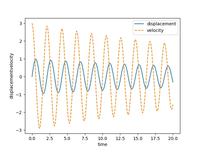
1) Initial displacement is zero, so that starts from zero corresponds to zero seconds. Over the period of time, an oscillation was shrinkage due to the damping ratio on that simple pendulum.

2) Initial velocity is three, so that starts from three corresponds to zero seconds. Over the period of time, velocity also was shrinkage due to decreasing the angular displacement on that simple pendulum.

3) Angular velocity is proportional to angular displacement

-->Output Graph

-->Output VIDEO