Compute 4th order approximations of the second-order derivative using various schemes to understand truncation error variation.

Compute 4th order approximations of the second-order derivative using various schemes to understand truncation error variation.

Aim:

To write and execute a MATLAB program for 4th order approximations of the second order derivative using Taylor's Table method of the function exp(x)*cos(x) and compare the results with central difference and skewed schemes.

Theory:

For the same mesh, we can get better accuracy, reduced number of mesh points, reduced computational time and storage. Therefore, any computational that requires resolution of small length scales(i.e. important physics occurs at small length scales) or has very sharp spatial gradients is an ideal candidate for higher order differencing.

examples includes:

• Direct Numerical simulation (DNS) of turbulent flow.
• Large Eddy Simulation (LES) of turbulent flow.
• Electromagnetic calculation (Maxwell Equation)

In this demostration we will evaluate the 4th order approximation of diffrent schemes for second derivative of the function exp(x)*cos(x) and

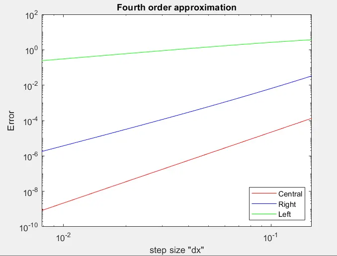
• plot that will compare the absolute errors between the schemes,
• comparision of the errors with FDS abd BDS approximations
• To conclude, how skewed schemes are useful and benifit of it than central scheme
• MATLAB codes with required functions

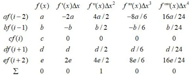
Formulation for the Taylor table methos for CDS

f''(x)=(af(x-2h)+bf(x-h)+cf(x)+df(x+h)+e(x+2h))/h^2

Formulation for the Taylor table method of left Skewed schme

f''(x) = (af(x)+bf(x-h)+cf(x-2h)+df(x-3h)+ef(x-4h)+ff(x-5h))/h^2

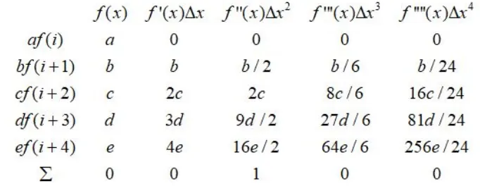
Formulation for the Taylor table method of Right-Skewed schme

f''(x)= (af(x)+bf(x+h)+cf(x+2h)+df(x+3h)+ef(x+4h)+ff(x+5h))/h^2

Central difference scheme

Right sided skewed scheme

Left sided skewed scheme

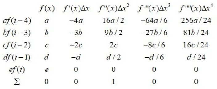
The Taylor's Table is made by expanding the well known Taylor's Series. In above equations we need to find the coefficients a,b,c,d and e for each schemes by comparing the coefficents of taylor's Series expansion to LHS. To make our life little easier, I have inserted the MATLAB program for execution of these coeffiicients.

When solving: by X=AB, we get the following results for different schemes'

1. 4th order CDS

a=-0.0833 b=1.333 c=-2.5 d=1.3333 e=-0.8333

2. 4th order Right sided skewed scheme

a=2.91667 b=-8.6667 c=9.5 d=-4.6667 e=0.91667

3. 4th order Left sided skewed scheme

a=0.91667 b=-4.6667 c=9.5 d=-8.6667 e=2.9167

Code:

Main code

clear all
close all
clc

x = pi/3;
dx= linspace(pi/20,pi/400,20);     
%dx= linspace(0.01,1,15);
for i=1:length(dx)
    [cen_error,right_error,left_error] = central(x,dx(i));
    err_central(i) = cen_error;
    err_right(i) = right_error;
    err_left(i) = left_error;
end

loglog(dx,err_central,'r');
hold on
loglog(dx,err_right,'b');
hold on
loglog(dx,err_left,'g');
hold off
title('Fourth order approximation');
xlabel('step size "dx"');
ylabel('Error')
legend('Central','Right','Left','Location','southeast')

Calculating errors for each schemes

function [cen_error,right_error,left_error] = central(x,dx)
analytical_derivative = -2*sin(x)*exp(x);
[X,Y,Z]=coeff_calc();
%numerical derivative
central_diff = ((X(1)*cos(x-2*dx)*exp(x-2*dx))+(X(2)*cos(x-dx)*exp(x-dx))+(X(3)*cos(x)*exp(x))+(X(4)*cos(x+dx)*exp(x+dx))+(X(5)*cos(x+2*dx)*exp(x+2*dx)))/dx^2;
cen_error = abs(analytical_derivative - central_diff);

right_diff = ((Y(1)*cos(x)*exp(x))+(Y(2)*cos(x+dx)*exp(x+dx))+(Y(3)*cos(x+2*dx)*exp(x+2*dx))+(Y(4)*cos(x+3*dx)*exp(x+3*dx))+(Y(5)*cos(x+4*dx)*exp(x+4*dx)))/dx^2;
right_error = abs(analytical_derivative - right_diff);

left_diff = ((Z(1)*cos(x)*exp(x))+(Z(2)*cos(x-dx)*exp(x-dx))+(Z(3)*cos(x-2*dx)*exp(x-2*dx))+(Z(4)*cos(x-3*dx)*exp(x-3*dx))+(Z(5)*cos(x-4*dx)*exp(x-4*dx)))/dx^2;
left_error = abs(analytical_derivative - left_diff);
end

Calculating coefficients for each scheme

function [X, Y, Z] = coeff_calc()
%calculate coefficients
%central
A=[1 1 1 1 1; -2 -1 0 1 2;4/2 1/2 0 1/2 4/2; -8/6 -1/6 0 1/6 8/6; 16/24 1/24 0 1/24 16/24];
B= [0;0;1;0;0];
X= inv(A)*B;

%right
A=[1 1 1 1 1;0 1 2 3 4;0 1/2 2 9/2 16/2;0 1/6 8/6 27/6 64/6;0 1/24 16/24 81/24 256/24];
B=[0;0;1;0;0];
Y= inv(A)*B;


%left
A=[1 1 1 1 1;-4 -3 -2 -1 0;16/2 9/2 2 1/2 0;-64/6 -27/6 -8/6 -1/6 0;256/24 81/24 16/24 1/24 0];
B=[0;0;1;0;0];
Z= inv(A)*B;
end

Result:

Conclusion:

As seen on the above plot, the central differencing scheme has very less error compared to other schemes, obviously it gathers informations from both neihbouring nodes. Skewed achemes are useful to calculate the values near to boundary where a central differencing cannot be used due to absence of terms away from boundary.