Effect of fluid property on Rayleigh Taylor Instability
Effect of fluid property on Rayleigh Taylor Instability
Aim: To simulate Rayleigh Taylor instability using different mesh size and using different fluid properties.
Case1: 0.5 element size (water and air)
Case2: 0.1 element size(water and air)
Case3: Using water and user-defined material(density = 400 kg/m3, viscosity = 0.001 kg/m-s) for refined mesh
Theory:
- What are some practical CFD models that have been based on the mathematical analysis of Rayleigh Taylor waves? In your own words, explain how these mathematical models have been adapted for CFD calculations.
The Rayleigh–Taylor instability, or RT instability (after Lord Rayleigh and G. I. Taylor), is an instability of an interface between two fluids of different densities which occurs when the lighter fluid is pushing the heavier fluid. Examples include the behavior of water suspended above oil in the gravity of Earth, mushroom clouds like those from volcanic eruptions and atmospheric nuclear explosions,supernova explosions in which expanding core gas is accelerated into denser shell gas,instabilities in plasma fusion reactors and inertial confinement fusion.
CFD models
Turbulence mixing models can be classified into three categories. The simplest models are called buoyancy drag models and use ordinary differential equations to evolve the width of the mixing layer. The bubble, or spike, amplitudes are described by balancing the inertia, buoyancy, and drag forces. These models cannot model multiple mixing interfaces; cannot be easily extended to two and three dimensions; and, as a rule, do not address demixing, also known as countergradient transport, i.e., reduction of total fluid masses within the mixing zone.
To address the above problems, twofluid (or multi-fluid) models have been proposed. They use a separate set of equations for each fluid in addition to the main flow equations and provide an accurate modeling framework for demixing by correctly capturing the relative motion of the different fluid fragments.
An intermediate class of models are the single-fluid models . They consist of evolutionary equations for the turbulence kinetic energy and its dissipation rate or equivalent turbulence length scale. A more advanced version of the single-fluid models is the Besnard-Harlow-Rauenzahn (BHR) model . The BHR model is based on the evolution equations arising from second-order correlations and gradient-diffusion approximations. Using a mass-weighted averaged decomposition, the original BHR model includes full transport equations for the Reynolds stresses, turbulent mass-flux velocity, density fluctuations, and the turbulence kinetic energy dissipation rate. Several efforts were made to simplify the resulting equations.
A three-equation variant was proposed for RT, KelvinHelmholtz (KH), and Richtmyer-Meshkov (RM) flows. A second-moment closure implementation was also presented by Schwarzkopf et al.. In the present study, the fourequation variant, known as the BHR-2 model, was employed. The BHR-2 model is also investigated here in conjunction with the modified species turbulent diffusion term, which can improve accuracy in demixing
Procedure:
1. Space claim is opened and the geometry is drawn using the sketch command and surfaces are created using the pull tool.
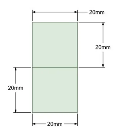
2. The two parts are combined using the share topology tool
3. Two different cases of mesh are created Case 1 : 0.5 mm mesh size and Case 2 : 0.3 mm mesh size
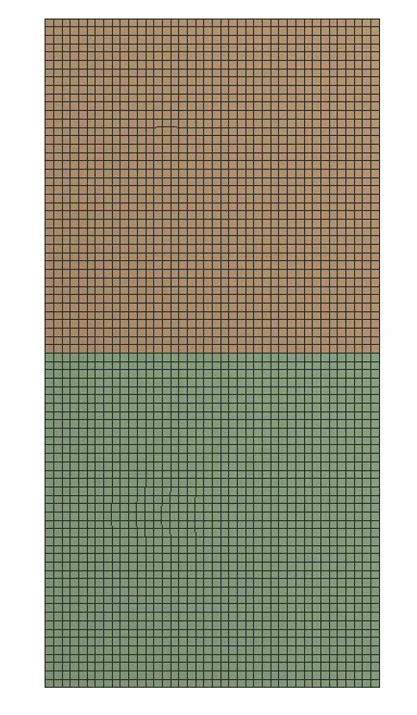
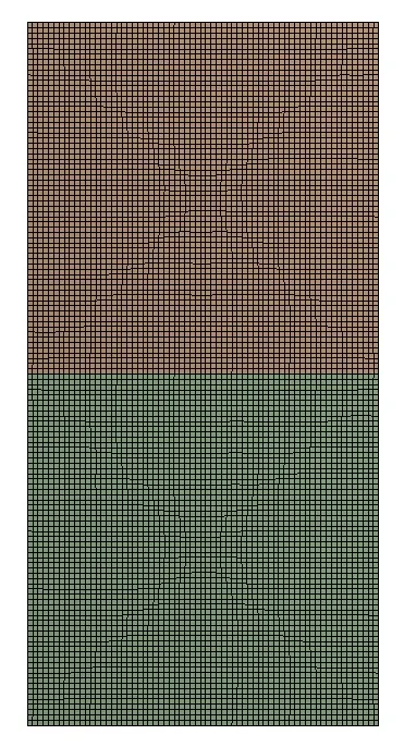
4. Inside Setup three different materials are defined namely air, water and a material with density =400 kg/m3 and viscosity = 0.001 kg/ms
5. In mutiphase below properties are defined
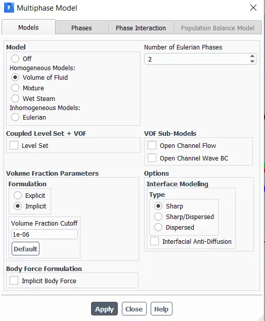
6. In solution tab initialization is done and then patch option is used to patch the material card to each of their respective surfaces.
Water is given a value =1 and air =0. The below contour will be obtained.
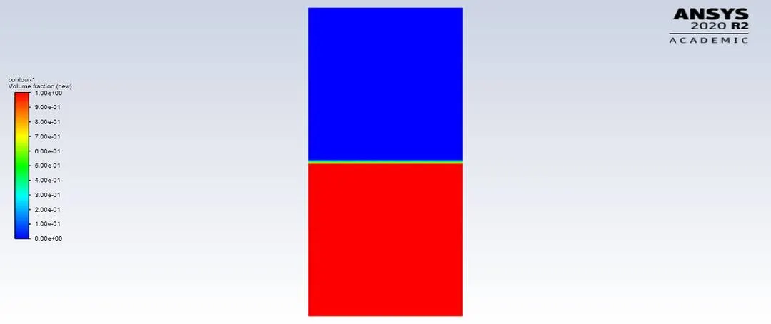
7. The solution is run for a time step size =0.005 and number of time steps = 1500
Results:
Case 1:
As seen in above simulation the values are slightly distorted due to large size of the mesh. The result obtained is not accurate because of the coarsness of the mesh.
Case 2:
When using a refined mesh the actula Rayleigh Taylor instability can be visualized as above. The minute details missing in the initial base line mesh is clearly visible in the above refined case.
Case 3:
Here since we are using a denser fluid than air the mixing happens slowly so the instability can be seen to be developing at a slower rate.
Atwood number: The Atwood number (A) is a dimensionless number in fluid dynamics used in the study of hydrodynamic instabilities in density stratified flows. It is a dimensionless density ratio defined as
`A = (rho_1-rho_2)/(rho_1+rho_2)`
where
`rho_1 =` density of heavier fluid
`rho_2=` density of lighter fluid
In Case 1 and Case 2
`rho_1 =` 998.2 kg/m3
`rho_2=` 1.225 kg/m3
A = 0.99755
In Case 3
`rho_1 =` 998.2 kg/m3
`rho_2=` 400 kg/m3
A = 0.42783
In Rayleigh–Taylor instability, the penetration distance of heavy fluid bubbles into the light fluid is a function of acceleration time scale, `A*g*t^2` where g is the gravitational acceleration and t is the time.
So in cases 1 and 2 where Atwood number is high the penetration will be high and in case 3 with lesser Atwood number the penetration distance is less as seen from the animation files.