Conjugate heat transfer analysis of an Exhaust port
Conjugate heat transfer analysis of an Exhaust port
Aim:
To study the CHT behaviour of exhaut port and to do a grid independence test
Theory:
Computational Fluid Dynamics (CFD) and more specifically conjugate heat transfer (CHT) analysis can accurately predict heat transfer by simultaneous solving all the relevant solid and flow field heat transfer processes, for example: conduction through solids, free and forced convection in the gases/fluids and thermal radiation.
The CHT approach has an advantage over FE thermal analyses in that wall heat transfer coefficients and their local variations on surfaces are directly calculated within the model rather than based on simplified empirical calculations. The CHT approach therefore has benefits for those applications where heat transfer is either non-uniform or difficult to calculate empirically.
Starting from simple examples in the 1960s, the conjugate heat transfer methods have become a more powerful tool for modeling and investigating nature phenomena and engineering systems in different areas ranging from aerospace and nuclear reactors to thermal goods treatment and food processing, from complex procedures in medicine to atmosphere/ocean thermal interaction in meteorology, and from relatively simple units to multistage, nonlinear processes.
Procedure:
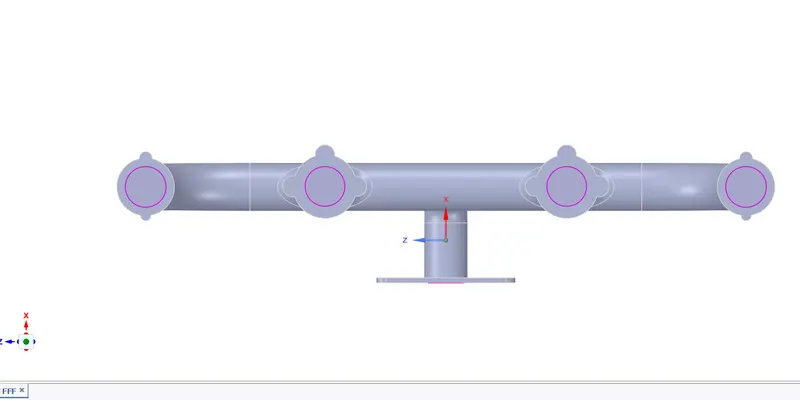
1. The geometry is loaded into Spaceclaim. Repair option is used to remove any duplicate edges. Using the volume extract the inside fluid vlume is extracted. Using the fluid and solid volume a new component is created. Topology sharing is turned on and the geometry looks as below.
2. The two cases are used for meshing
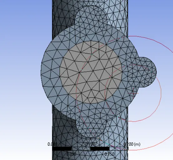
Case 1 : Baseline mesh of 150 mm, no infaltion layers
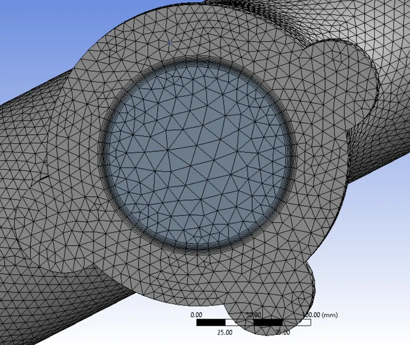
Case 2 : solid element size = 10mm, inflation layer of 5mm applied to fluid volume
3. In the Setup tab below conditions are provided
Solver type - Pressure Based steady state solver
Viscous model - K-Epsilon standard with Energy equation ON.
Material - Fluid : Air; Solid : Aluminium
Inlet BC - Velocity = 5 m/s; Temperature = 700K
Outer Wall - Thermal Conditions = Convection; Heat Transfer Coefficient = 20 W/m^2K; Free Stream Temperature = 300K.
4. The simulation is run for 150 iterations and the results are plotted in CFD post
Results:
Case 1 : Baseline mesh of 150 mm, no infaltion layers
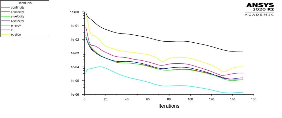
The residual plots show a steady decrease showing the solution is converging
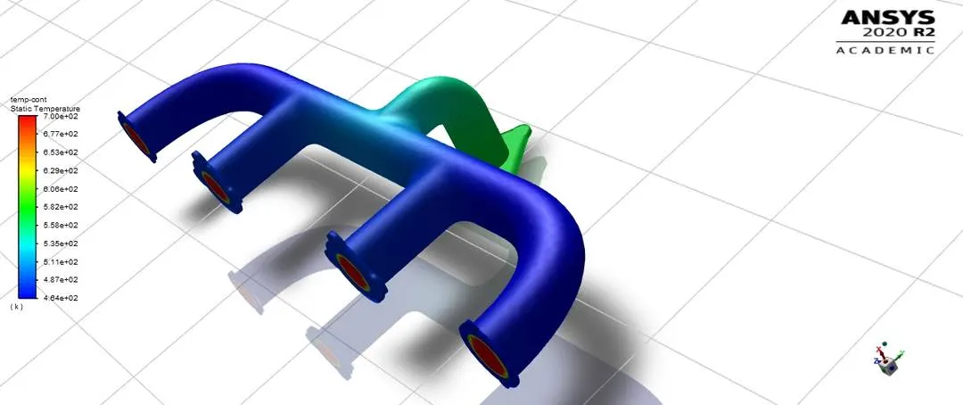
The below temperature contours show that the temperature is higher at the outlet section (538K) and lower at inlet section (433K) eventhough the inlet temperature is 700K. This is beacuse of higher convective coefficient at the outlet section due to higher rate of flow.
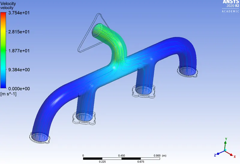
The velocity can be seen as higher in the outlet section because of mass conservation.
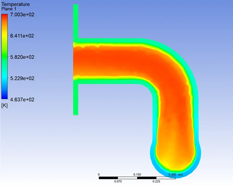
Outlet temperature distribution is as shown below.
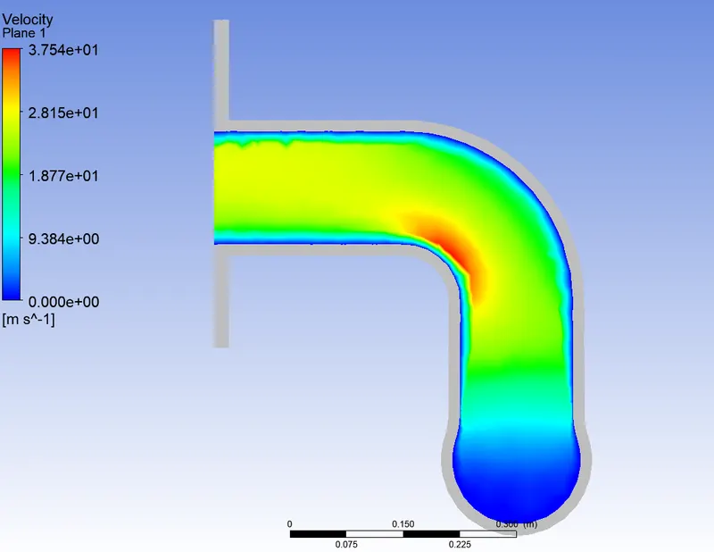
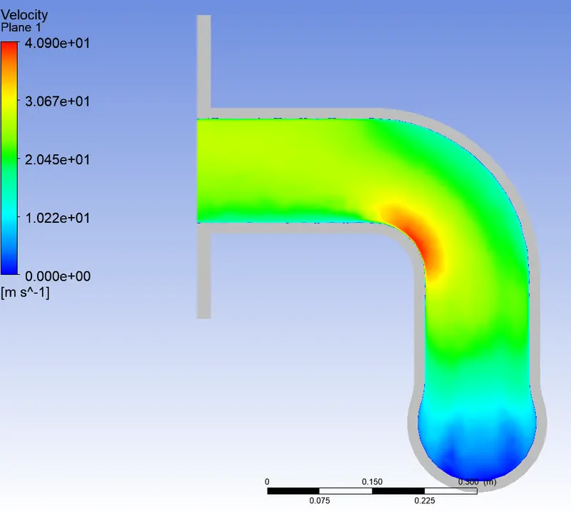
Outlet velocity distribution is as shown below. It can be seen that the velocity is higher near the bend section.
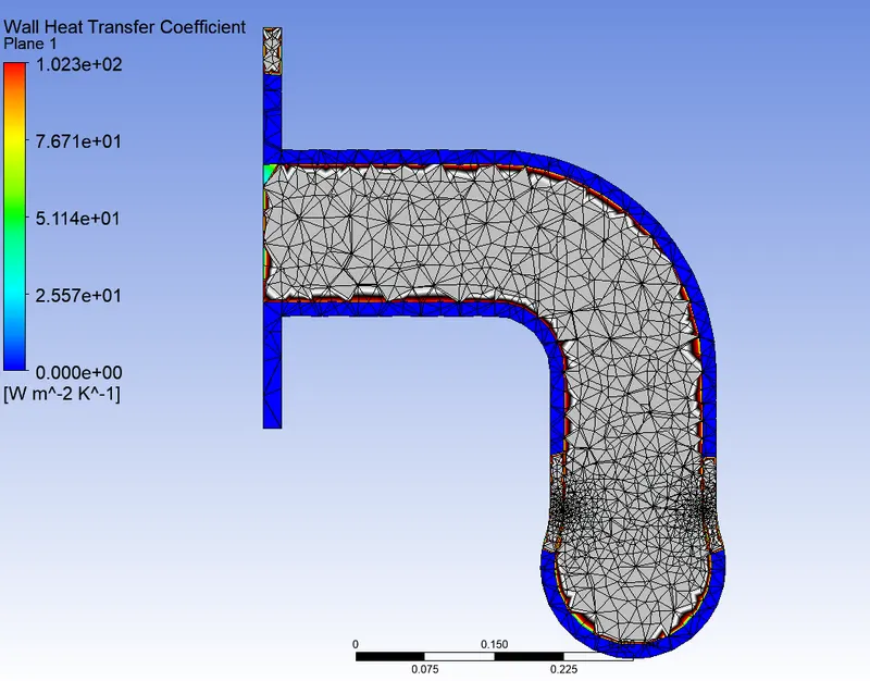
Because of higher velocity in the bend section the wall heat transfer coefficient can be seen to be higher in that section. Moreover due to coarser mesh the coefficient value is seen to be slightly distributed near the wall section.
Case 2 : solid element size = 10mm, inflation layer of 5mm applied to fluid volume
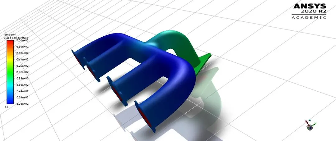
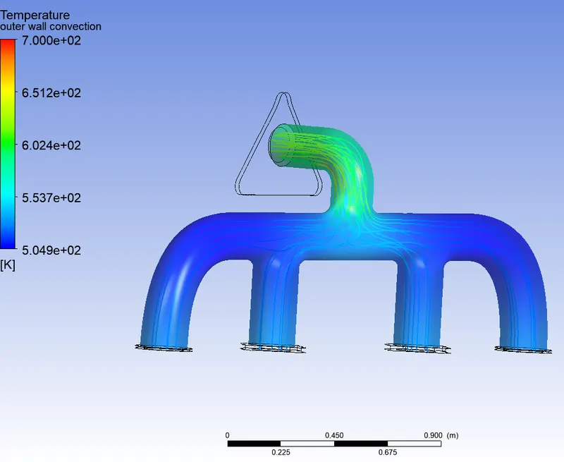
The temperature contour looks similar to that of coarser mesh with only slight change in the temperature values.
Outlet temperature distribution is as shown below.
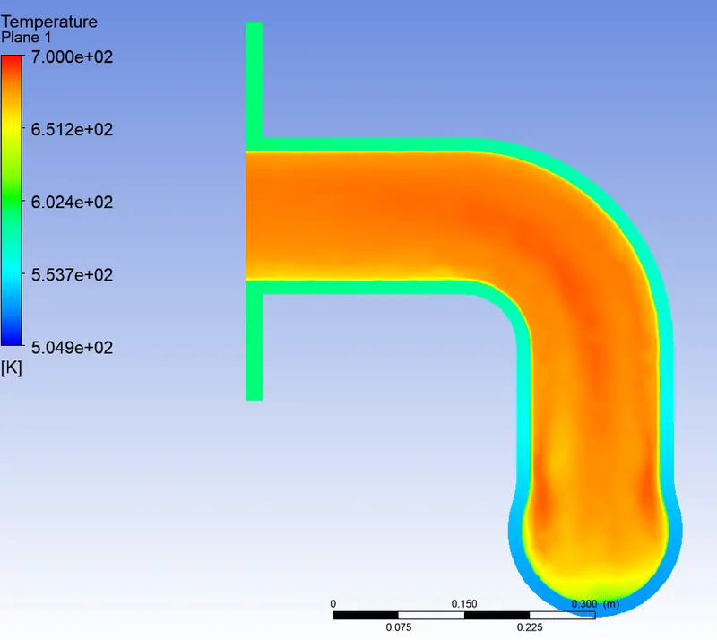
Outlet velocity distribution is as shown below.
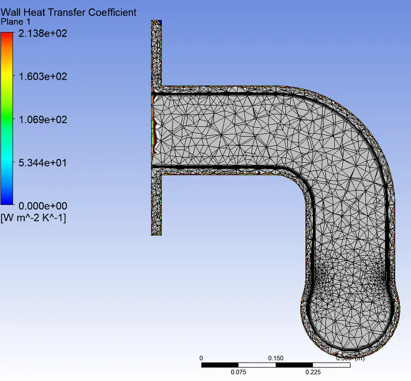
When a finer mesh is used with an inflation layer the heat transfer coefficient is seen to be sticking very close to the wall which is the proper result required.
Conclusion:
The element size has a significant effect on the wall heat transfer coefficient. The contour looks similar but there is a slight variation between the temperature and velocity of flow obtained aas seen in below table.
Parameters Case 1 Case 2
Max. wall temperature(K) 601.5 602.7
Max. Velocity(m/s) 37.54 40.9
Wall HTC (W/m^2K) 102.3 213.8
- Verification of HTC
Heat transfer coefficient can be verified by using Nusselt number.
Nusselt Number is given by
`Nu=0.023*(Re)^(4/5)*(Pr)^0.4`
Re increases with increase in velocity which in turn will increase Nusselt number.
also, `Nu=(h*l)/k`
Meaning when velocity increases, convective heat transfer will also increase.
- Factors affecting simulation :
- Number of elements and element size of the mesh :- Finer mesh will give accurate results
- Inflation layers provide better wall coefficients closer to the boundary.
- Proper fitting of mesh around the curvature
- Selection of material and its properties. Here we used air and aluminium.
- If there is multiple zones mesh sharing should be done so that there will be smooth transistion.