Week 7 - Simulation of a 1D Super-sonic nozzle flow simulation using Macormack Method
Isentropic flow simulation through a quasi 1D subsonic-supersonic nozzle
Aim:
To solve the quasi 1D nozzle flow simulation using Maccormack method for conservative and Non conseravative forms of the governing equation
Procedure:
The schematic of nozzle is as shown below. The flow at inlet comes from the reservoir. The cross sectional area of the reservoir is large so pressure and temperature are stagnation values. The flow is subsonic in the convergent section of the nozzle, sonic at the throat(minimum area), and supersonic at the divergent section.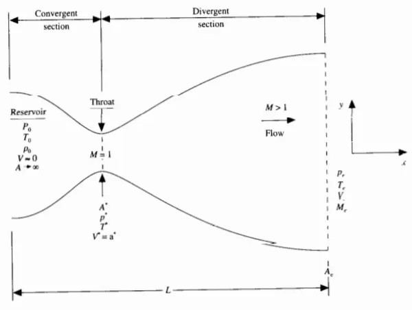
Governing eequations are as given below.
Non conservative form
Continuity equation
`(∂ ρ ')/ (∂ t ') = ρ( ' ∂ V )/(' ∂ x ' )− ρ ' V ' (∂ ( ln A ))/( ∂ x ' )− V '( ∂ p ')/( ∂ x ')`
Momentum Equation
`(∂ V ')/( ∂ t ') = V '( ∂ V')/( ∂ x ') − 1 /γ (( ∂ T ' ) / (∂ x ') + (T ')/ (ρ ')( ∂ ρ ')/( ∂ x '))`
Energy equation
`(∂ T ')/( ∂ t ') =( V ' )(∂ T ' )/(∂ x ') − ( γ − 1 ) T ' [ (∂ V ')/( ∂ x ') + V '( ∂ ( ln A ' ))/( ∂ x ' )]`
Conservative form
Continuity equation
`(∂ ( ρ ' A ' )) /(∂ t ' )+ (∂ ( ρ ' A ' V ' ) )/(∂ x ') = 0`
Momentum Equation
`(∂ ( ρ ' A ' V ' ) )/(∂ t ') + (∂ ( ρ ' A ' V ' 2 + 1 /γ p ' A ' ) )/(∂ x ') = 1 /γ p ' (∂ A ')/( ∂ x ')`
Energy equation
`( ∂[ ρ ' ( (T ')/( γ − 1 )+ γ /2 V ' ^2 ) A ' ]) /(∂ t ') + (∂ [ ρ ' ( T ')/( γ − 1 )+ γ /2 V ' ^2 ) V ' A ' + p ' A ' V ' ] /(∂ x ' )= 0`
Calculation of time step
We use Courant number C<1 .
`Delta t=C(Delta x)/(a+V)`
We calculate this at all the grid points for all time step value and the minimum value is taken into consideration.
MacCormacks method
1. Initialize all the variables
2. Use predictor method to calculate all the differential derivative in the governing equations
3. Update the solution
4. Use corrector method to calculate all the differential derivative in the governing equations
5. Find the average of corrector and predictor derivatives
6. Update the solution for last time
7. Repeat above steps till convergence
Matlab code:
Main
clear all
close all
clc
 [x,V,T,P,rho,m,M,M_throat,rho_throat,P_throat,T_throat]=nozzle_nonconservative;

 [xc,Vc,Tc,Pc,rhoc,mc,Mc,Mc_throat,rhoc_throat,Pc_throat,Tc_throat]=nozzle_conservative;

 figure(1)
subplot(4,1,1)
plot(x,M)
hold on
plot(xc,Mc,'*')
ylabel('Mach number');
xlabel('x');
title('Mach number variation');
legend('Non-Conservative form', 'Conservative form');
subplot(4,1,2)
plot(x,rho)
hold on
plot(xc,rhoc,'*')
ylabel('rho/rho_o');
xlabel('x');
title('Non dimensional density variation');
legend('Non-Conservative form', 'Conservative form');
subplot(4,1,3)
plot(x,P)
hold on
plot(xc,Pc,'*')
ylabel('P/Po');
xlabel('x');
title('Non dimensional pressure variation');
legend('Non-Conservative form', 'Conservative form');
subplot(4,1,4)
plot(x,T)
hold on
plot(xc,Tc,'*')
ylabel('T/To');
xlabel('x');
title('Non dimensional temperature variation');
legend('Non-Conservative form', 'Conservative form');

t=1:1000;
figure(2)
subplot(4,1,1)
plot(t,M_throat)
hold on
plot(t,Mc_throat)
ylabel('Mach number');
xlabel('time');
title('Mach number variation at throat with respect to simulation time');
legend('Non-Conservative form', 'Conservative form');
subplot(4,1,2)
plot(t,rho_throat)
hold on
plot(t,rhoc_throat)
ylabel('rho/rho_o');
xlabel('time');
title('Non dimensional density variation at throat with respect to simulation time');
legend('Non-Conservative form', 'Conservative form');
subplot(4,1,3)
plot(t,P_throat)
hold on
plot(t,Pc_throat)
ylabel('P/Po');
xlabel('time');
title('Non dimensional pressure variation at throat with respect to simulation time');
legend('Non-Conservative form', 'Conservative form');
subplot(4,1,4)
plot(t,T_throat)
hold on
plot(t,Tc_throat)
ylabel('T/To');
xlabel('time');
title('Non dimensional temperature variation at throat with respect to simulation time');
legend('Non-Conservative form', 'Conservative form');

figure(3)
plot(x,m)
hold on
plot(xc,mc)
ylabel('mass flow rate');
xlabel('x');
title('Mass flow rate variation in nozzle');
legend('Non-Conservative form', 'Conservative form');
Non conservative form code
function[x,V,T,P,rho,m,M,M_throat,rho_throat,P_throat,T_throat]=nozzle_nonconservative()

%inputs
n=31;
x=linspace(0,3,n);
dx=x(2)-x(1);

%Initial profiles
rho=1-0.3146*x;
T=1-0.2314*x;%temperature
V=(0.1+1.09*x).*T.^0.5;
A=1+2.2*(x-1.5).^2;%area
gamma =1.4;
C=0.5;

%time steps
nt=1000;

%outer time loop
for k=1:nt

    dt=min(C*dx./(sqrt(T) + V));

    %predictor method
    rho_old=rho;
    V_old=V;
    T_old=T;

    for j=2:n-1
        %d_rho_dt(j)=-rho(j)*(v(j+1)-v(j))/dx - rho(j)*v(j)*(log(a(j+1))-log(a(j)))/dx - v(j)*(rho(j+1)-rho(j))/dx;
        dvdx = (V(j+1)-V(j))/dx;
        drhodx = (rho(j+1) - rho(j))/dx;
        dTdx = (T(j+1)-T(j))/dx;
        dlog_a_dx = (log(A(j+1))-log(A(j)))/dx;
        %Continuity Equation
        drhodt_p(j) = -rho(j)*dvdx - rho(j)*V(j)*dlog_a_dx -V(j)*drhodx;
        % Momentum Equation
        dvdt_p(j) = -V(j)*dvdx - (1/gamma)*(dTdx + (T(j)/rho(j))*drhodx);
        % Energy Equation
        dTdt_p(j) = -V(j)*dTdx - (gamma-1)*T(j)*(dvdx + V(j)*dlog_a_dx);

        %Solution update
        rho(j) = rho(j) + drhodt_p(j)*dt;
        V(j) = V(j) + dvdt_p(j)*dt;
        T(j) = T(j) + dTdt_p(j)*dt;
    end

    %corrector step
for j=2:n-1
        dvdx = (V(j)-V(j-1))/dx;
        drhodx = (rho(j) - rho(j-1))/dx;
        dTdx = (T(j) - T(j-1))/dx;
        dlog_a_dx = (log(A(j))-log(A(j-1)))/dx;

        drhodt_c(j) = -rho(j)*dvdx - rho(j)*V(j)*dlog_a_dx - V(j)*drhodx;

        dvdt_c(j) = -V(j)*dvdx - (1/gamma)*(dTdx + (T(j)/rho(j))*drhodx);

        dTdt_c(j) = -V(j)*dTdx - (gamma-1)*T(j)*(dvdx + V(j)*dlog_a_dx);

end

%Compute average time derivative
    drhodt = 0.5*(drhodt_p + drhodt_c);
    dvdt = 0.5*(dvdt_p + dvdt_c);
    dTdt = 0.5*(dTdt_p + dTdt_c);

    %Final solution update
for i = 2:n-1
        rho(i) = rho_old(i) + drhodt(i)*dt;
        V(i) = V_old(i) + dvdt(i)*dt;
        T(i) = T_old(i) + dTdt(i)*dt;
end
     % Applying BC
    % Inlet BC
    V(1) = 2*V(2) - V(3);
    rho(1) = 1;
    T(1) = 1;
    % Outlet BC
    V(n) = 2*V(n-1) - V(n-2);
    rho(n) = 2*rho(n-1) - rho(n-2);
    T(n) = 2*T(n-1) - T(n-2);
    P = rho.*T; % calculating Pressure
    M = V./sqrt(T);% calculating Mach
    m = rho.*A.*V;% calculating mass flow rate

     M_throat(k)=M(16);
         rho_throat(k)=rho(16);
       P_throat(k)=P(16);
       T_throat(k)=T(16);
%     plot(x,V);
%     title(sprintf('Time step=%d',k))
%     pause(0.03);

figure(5);
    hold on;
    if          k == 1
                plot(x,m,'b','linewidth',1.5);

                elseif k == 100
                plot(x,m,'g','linewidth',1.5);

                elseif k == 200
                plot(x,m,'c','linewidth',1.5);

                elseif k == 700
                plot(x,m,'y','linewidth',1.5);
                legend('t=0','t=100','t=200','t=700');
                xlabel('x');
                ylabel('mass flow rate')
                title('Non-conservative')

    end

end
Conservative form code
function[x,V,T,P,rho,m,M,M_throat,rho_throat,P_throat,T_throat]=nozzle_conservative()

%inputs
n=31;
x=linspace(0,3,n);
dx=x(2)-x(1);

%Initial profiles
for i = 1:n
    if x(i) >= 0 && x(i) < 0.5
        rho(i) = 1;
        T(i) = 1;
    elseif (x(i) >= 0.5 && x(i) < 1.5)
            rho(i) = 1.0 -0.366*(x(i) - 0.5);
            T(i) = 1.0 - 0.167*(x(i) - 0.5);
    elseif (x(i) >= 1.5 && x(i) <= 3.0)
                rho(i) = 0.634 - 0.3879*(x(i) - 1.5);
                T(i) = 0.833 - 0.3507*(x(i) - 1.5);
    end
end
A=1+2.2*(x-1.5).^2;%area

% Velocity and Pressure Initialise
V = 0.59./(rho.*A);
P = rho.*T;
C=0.5;
gamma =1.4;

%U1,U2,U3
U1 = rho.*A;
U2 = rho.*A.*V;
U3 = rho.*A.*((T./(gamma - 1)) + (gamma/2)*V.^2);

%time steps
nt=1000;

%outer time loop
for k=1:nt

    %dt=0.001;
    dt=min(C*dx./(sqrt(T) + V)); %optimum vaue of time step using courant number


    U1_old = U1;
    U2_old = U2;
    U3_old = U3;

    F1 = U2;
    F2 = (U2.^2./U1) + ((gamma-1)/gamma)*(U3 - (gamma*U2.^2)./(2*U1));
    F3 = (gamma*U2.*U3./U1) - (gamma*(gamma-1)/2)*(U2.^3./U1.^2);

    %predictor method
    for j=2:n-1
        J2(j)=rho(j)*T(j)*(A(j+1)-A(j))/(dx*gamma);
        %continuity equation
        dU1dt_p(j) = -(F1(j+1) - F1(j))/dx;
        %momentum equation
        dU2dt_p(j) = -((F2(j+1) - F2(j))/dx) + J2(j);
        %energy equation
        dU3dt_p(j) = -(F3(j+1) - F3(j))/dx;

        %first solution update
        U1(j) = U1(j) + dU1dt_p(j)*dt;
        U2(j) = U2(j) + dU2dt_p(j)*dt;
        U3(j) = U3(j) + dU3dt_p(j)*dt;
    end

     % Updating values of rho,V,T after predictor Step:
    rho = U1./A;
    V = U2./U1;
    T = (gamma -1)*(U3./U1 - (gamma/2)*V.^2);
    P = rho.*T;
    %Updating flux - corrector step
    F1 = U2;
    F2 = (U2.^2./U1) + ((gamma-1)/gamma)*(U3 - (gamma*U2.^2)./(2*U1));
    F3 = (gamma*U2.*U3./U1) - (gamma*(gamma-1)/2)*(U2.^3./U1.^2);

    %corrector method
    for j=2:n-1
        J2(j)=rho(j)*T(j)*(A(j)-A(j-1))/(dx*gamma);
        %continuity equation
        dU1dt_c(j) = -(F1(j) - F1(j-1))/dx;
        %momentum equation
        dU2dt_c(j) = -((F2(j) - F2(j-1))/dx) + J2(j);
        %energy equation
        dU3dt_c(j) = -(F3(j) - F3(j-1))/dx;
    end

    % Finding the average of predictor and corrector steps:
    dU1dt = 0.5*(dU1dt_p + dU1dt_c);
    dU2dt = 0.5*(dU2dt_p + dU2dt_c);
    dU3dt = 0.5*(dU3dt_p + dU3dt_c);

    %final solution update
    for j = 2:n-1
        U1(j) = U1_old(j) + dU1dt(j)*dt;
        U2(j) = U2_old(j) + dU2dt(j)*dt;
        U3(j) = U3_old(j) + dU3dt(j)*dt;
    end

    %boundary conditions
    U1(1) = rho(1)*A(1);
    U2(1) = 2*U2(2) - U2(3);
    V(1) = U2(1)/U1(1);
    U3(1) = U1(1)*((T(1)/(gamma-1))+((gamma/2)*V(1)^2));

    U1(n) = 2*U1(n-1) - U1(n-2);
    U2(n) = 2*U2(n-1) - U2(n-2);
    U3(n) = 2*U3(n-1) - U3(n-2);

    %calculating primitive variables
    rho = U1./A;
    V = U2./U1;
    T = (gamma -1)*(U3./U1 - (gamma/2)*V.^2);
    P = rho.*T; % calculating Pressure
    M = V./sqrt(T);% calculating Mach
    m = rho.*A.*V;% calculating mass flow rate

       M_throat(k)=M(16);
       rho_throat(k)=rho(16);
       P_throat(k)=P(16);
       T_throat(k)=T(16);
%     plot(x,V)
%     title(sprintf('time step=%d',k))
%     pause(0.03)

figure(4);
    hold on;
    if          k == 1
                plot(x,m,'b','linewidth',1.5);

                elseif k == 100
                plot(x,m,'g','linewidth',1.5);

                elseif k == 200
                plot(x,m,'c','linewidth',1.5);

                elseif k == 700
                plot(x,m,'y','linewidth',1.5);
                legend('t=0','t=100','t=200','t=700');
                xlabel('x');
                ylabel('mass flow rate')
                title('Conservative')
    end

end
Result:
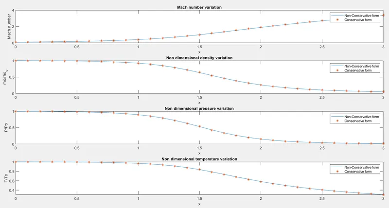
1. Below graph shows the non dimensional variation of density, pressure and temperature variation along the nozzle length
Mach number becomes sonic at throat section at length 1.5 as seen in graph below.
The below graph matches with the values given in the book.
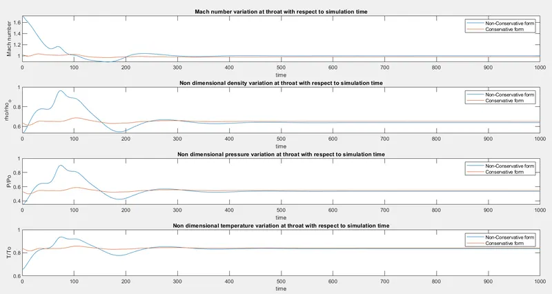
2. Variation of Mach number, non dimensional values of density, pressure and velocity for conservative and non conservative forms with respect to time steps.
The Mach number in non conservative form becomes steady at 1 at the throat section but for the conservative form the Mach number is slightly low at around 0.98.
The values become steady after 400 time steps.
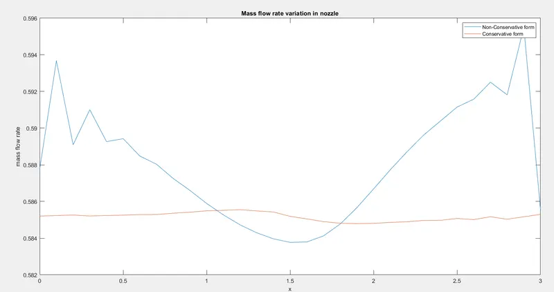
3. Mass slow rate variation through the nozzle for conservative and non conservative forms
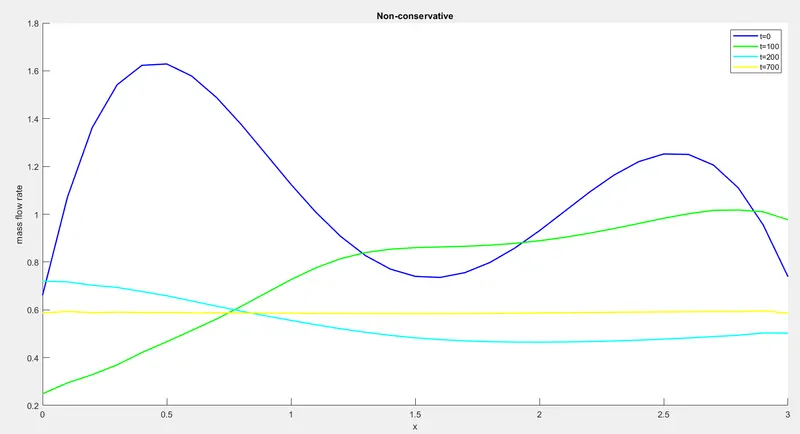
The conservation form does a better job of preserving mass throughout the flow field, mainly because the mass flow itself is one of the dependent variables in the equations-the mass flow is a primary result from these equations. In contrast, the dependent variables in the nonconservation form of the equations are the primitive variables, and the mass flow is obtained only as a secondary result. Because the conservation form of the equations does a better
job of conserving mass throughout the flow field, we can begin to understand why they are labeled the conservation form.
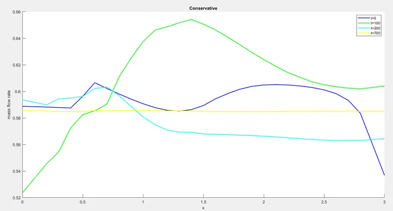
4. Conservative mass flow rate at different time steps
After 100 time steps, the mass flow distribution through the nozzle has changed considerably; this is given by the curve labeled t=100. After 100 time steps, the mass flow distribution has changed radically; the mass flow variation is simply flopping around inside the nozzle due to the transient variation of the flow-field variables. However, after 200 time steps, the mass flow distribution is beginning to settle down, and after 700 time steps, the mass flow distribution is a straight, horizontal line across the graph. This says that the mass flow has converged to a constant, steady-state value throughout the nozzle.
5. Non conservative mass flow rate at different time steps
6. Grid independence test
When increasing the grid size the solution accuracy incerases only a little bit which is considered negligible for this problem.
Conclusion:
Program is written using MacCormack method for solving both conservatiive and non conservative form.
The obtained result is compared with the actual and is found to be matching with exact solution.