Week 3 - Solving second order ODEs
AIM
write a program that solves the following ODE representing the equation of motion of a simple pendulum with damping.
This is to simulate the transient behaviour of a simple pendulum and create an animation of its motion.
INITIAL STUDY
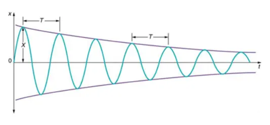
For a system that has a small amount of damping, the period and frequency are nearly the same as for simple harmonic motion, but the amplitude gradually decreases as shown in figure. This occurs because the non-conservative damping force removes energy from the system, usually in the form of thermal energy. In general, energy removal by non-conservative forces is described as
where  is work done by a non-conservative force (here the damping force). For a damped harmonic oscillator, is negative because it removes mechanical energy (KE + PE) from the system.
GOVERNING EQUATION
Second order differential equation governing the motion of a simple pendulum with natural damping is given as below:
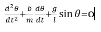
b=damping coefficient
m=mass (in kg)
g=acceleration due to gravity,m/s^2
l=length (in m)
#PROGRAM TO SIMULATE THE MOTION OF A SINGLE PENDULUM USING PYTHON
#CODE CREATED BY LAKSHMI RAJAN P
#CODED IN PYCHARM

#Importing the required modules
import math
import numpy as np
import matplotlib.pyplot as plt
#odeint is a function in scipy module which is used to perform integration of differential equations
from scipy.integrate import odeint

#The input values or the constants required to perform the differential equations are entered
print("The input values for the simulation of a single pendulum are as follows: ")
print('\n')
#m is mass in kilograms
m=1
print('mass of the pendulum ball,m in kg is ',m)
print('\t')
#l is the length of the pendulum string in meters
l=1
print('length of the pendulum string in meter is ',l)
print('\t')
#b is the damping coefficient
b=0.07
print('damping coefficient is ',b)
print('\t')
#g is the acceleration due to gravity in m/s^2
g=9.81
print('acceleration due to gravity, in m/s^2 is ',g)
print('\t')
#The initial angular displacement value is assigned as 0 rad and angular velocity to be 3 rad/sec
Y0=[0,3]
print('The initial values of angular displacement and angular velocity are ',Y0)
print('\n')
#The time span is set for 20sec
time_span=np.linspace(0,20,1000)
print('The time interval is ',time_span)
print('\n')
#A function is defined by splitting the general pendulum equation into two first order equations,here theta means
#angular displacement and omega means angular velocity
def odefunc(Y0,time_span,m,l,b,g):
    theta=Y0[0]
    omega=Y0[1]
    dtheta_dt=omega
    domega_dt=(-b/m)*(omega)-(g/l)*(theta)
    dTHETA_dt=[dtheta_dt,domega_dt]
    return(dTHETA_dt)
#calling the function to perform the integration using odeint package in scipy module
results=odeint(odefunc,Y0,time_span,args=(m,l,b,g))

Angular_displacement=[]
Angular_velocity=[]
for i in range(0,len(results)):
    angdisplacement=results[i,0]
    Angular_displacement.append(angdisplacement)
    angvelocity=results[i,1]
    Angular_velocity.append(angvelocity)

#plotting the graph between angular displacement with time and angular velocity with time
plt.figure(1)
plt.plot(time_span,Angular_displacement,color='r',linewidth=2,label='Angular displacement')
plt.plot(time_span,Angular_velocity,color='b',linewidth=2,label='Angular velocity')
plt.legend()
plt.grid()
plt.savefig('Graph showing variation of Angular displacement and Angular velocity with time.png')
#inorder to create figures of each position and to create an animation,we save each figure and the figures are saved with the
#help of a counter variable ct
ct=1
for j in range(0,len(time_span)):
    theta=Angular_displacement[j]
    omega=Angular_velocity[j]
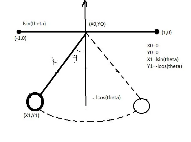
    #The initial values of the coordinates are assigned as below
    X0=0
    Y0=0
    X1=l*(math.sin(theta))
    Y1=-l*(math.cos(theta))
    plt.figure()
    #The coordinates of the support was mentioned as below to connect a line between the points
    plt.plot([-1,1],[0,0],linewidth=2,color='b')
    #A line is connected between the coordiantes of origin with the pendulum bob coordinates as below
    plt.plot([X0,X1],[Y0,Y1],linewidth=3,color='r')
    plt.plot(X1,Y1,marker='o',markerfacecolor='y',markeredgecolor='m',markersize=20)
    plt.grid()
    plt.title("SIMULATION OF MOTION OF SINGLE PENDULUM USING PYTHON")
    ct=ct+1
    filename=str(ct)+'.png'
    plt.savefig(filename)
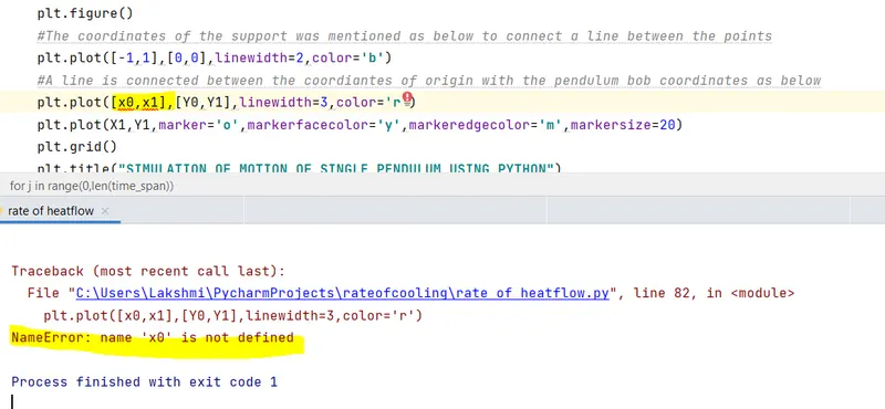
The x defined was small letter instead of capitals defined before.
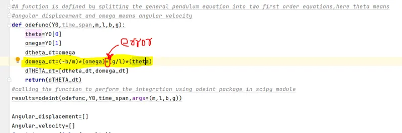
2)The graph was obtained in the opposite direction as the equation was mentioned with wrong sign in the omega equation
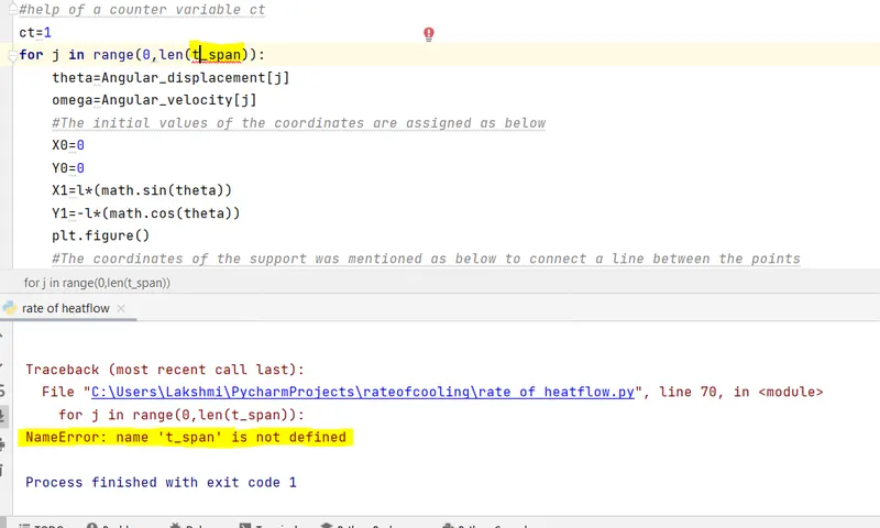
3)t_span was assigned instead of time_span.
Errors mentioned were clarified and ran again.
OUTPUT
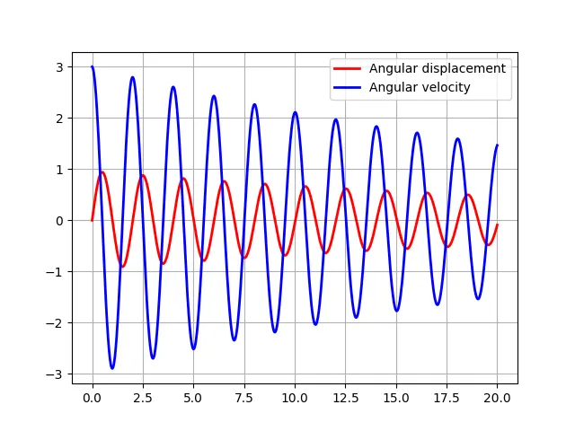
The graph showing the relationship between angular displacement and angular velocity were plotted.And increasing the damping coefficient values showed the vibrations reducing considerably.The problem on how to solve second order differential equations by dividing it to first order differential equations were studied.
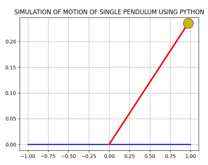
The animated motion of the simple pendulum is attached herewith.