Week 11 - Simulation of Flow through a pipe in OpenFoam
Date: - 26-02-2021
SIMULATION OF FLOW THROUGH A PIPE IN OPENFOAM
Laminar Flow in pipe: -
- Renold’s number is a non-dimensional number which is very important to describe the behaviour of flow whether it is internal or external flow.
- We deal with internal laminar flow through a pipe. Renold’s number is given as 2100.
- We have to find both analytical and numerical values for fully developed flow and compare the results.
Analytical solution for fully developed flow: -
- Before we find analytical solution, we should know about hydrodynamic length.
- In figure 1 we can see that with some input velocity the shear stress profile along the length of the pipe.
- If you go deeper the main reason for full developed flow is growing of boundary layers thickness until the mid-section of the pipe.
- Once it reaches mid-section of the pipe then in pipe we can see that the constant velocity profile that means
Consider x, r the independent coordinates then
From inlet of pipe to till hydrodynamic entry length
Velocity ‘u’ is function of both x,r u(x,r)
After hydrodynamic length
‘ u’ is function of ‘r’ only
ꝺu/ ꝺx = 0
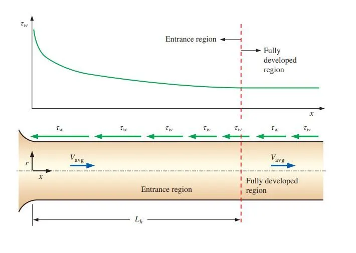
Fig(1)
- In figure 2 we can see that before hydrodynamic length variation of velocity profile with respect to length. Once it attains fully developed flow then we can observe constant velocity profile.
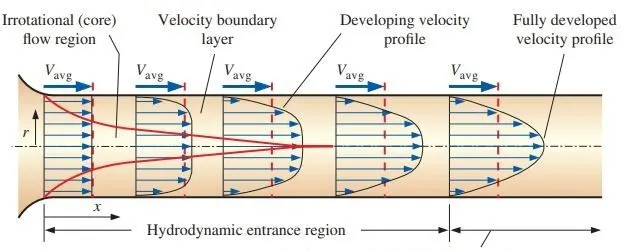
Fig(2)
- Mathematically we can say that Lh/D = 0.05 *Re for laminar flows
Where
Lh is hydrodynamic entry length
‘D’ is the hydralic diameter for circular pipe this is equal to diameter
- Consider one section in fully develop flow region and do force balance then we end up with
(μ/r)*d/dr(rdu/dr) = dp/dx ---1
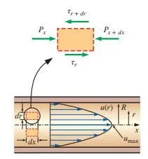
Fig(3)
- Form figure 4 we by force balancing we end up with
dp/dx = -2Γw/R -------2
where Γw = μ ꝺu/ ꝺr |wall which is constant for fully developed flow
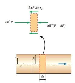
Fig(4)
- After integrating equation1 and limits from o to radius of pipe then we end up with
u(r) = 2*Vavg*(1-(r/R)2) ----3
where ‘r’ is the independent variable and ‘R’ is radius of the pipe
‘Vavg’ is the mean velocity of the full developed velocity profile.
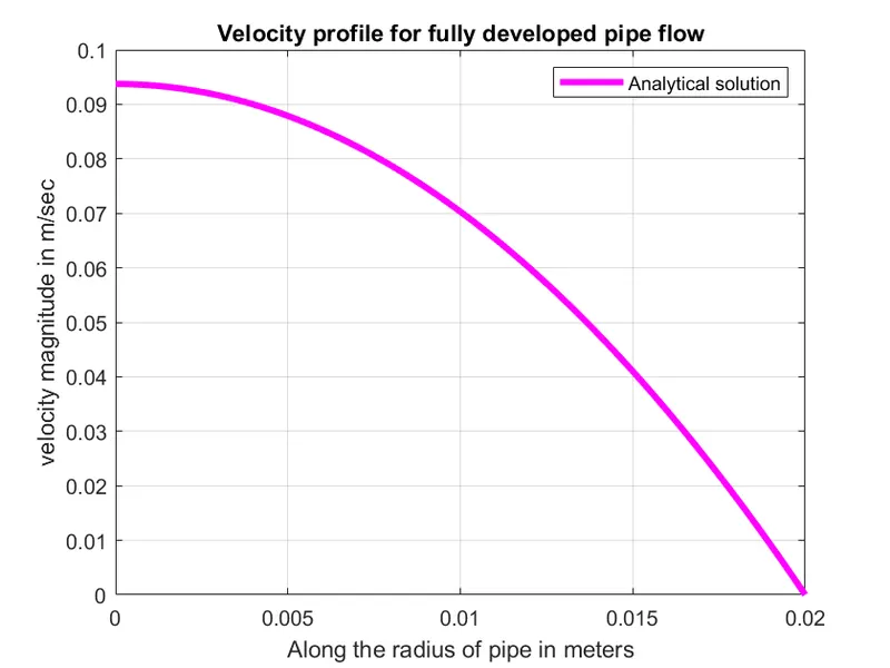
- Equation 3 is called Hagen- Poiseuille's equation for the fully developed flow.
Similarly for Maximum velocity Vmax = 2Vavg --4
Pressure difference Δp = 8 μ LVavg / r2 ----5
Kinematic pressure = Δp/ρ ------6
Shear stress Γ(r) = μ ꝺu/ ꝺr = 2μVmaxr/R ---7
Input Values:-
- Consider dimeter D=0.04 meters and given Renolds number Re = 2100.
- Density of water ρ = 997kg/m3 and dynamic viscosity of water μ = 0.00089 pa.sec
Outputs:-
- Then we can find Hyderodynamic entry length(Lh ) = 4.2 meters
- Total length (L) = Lh + 0.8 = 5 meters
Reason:-
- For know about the flow filed quantities in full developed ,length of pipe should be more than the hydrodynamic entry length so I took 5 meters as the legth of the pipe.
- Re = VavgD/ѵ where ѵ-kinematic viscosity
Then Vavg = 0.0468656 m/sec
- Vmax = 0.0937312 m/sec
- Pressure difference Δp = 4.1710384 pascals
- Kinematic pressure = 4.1835892*10-3m3/kg
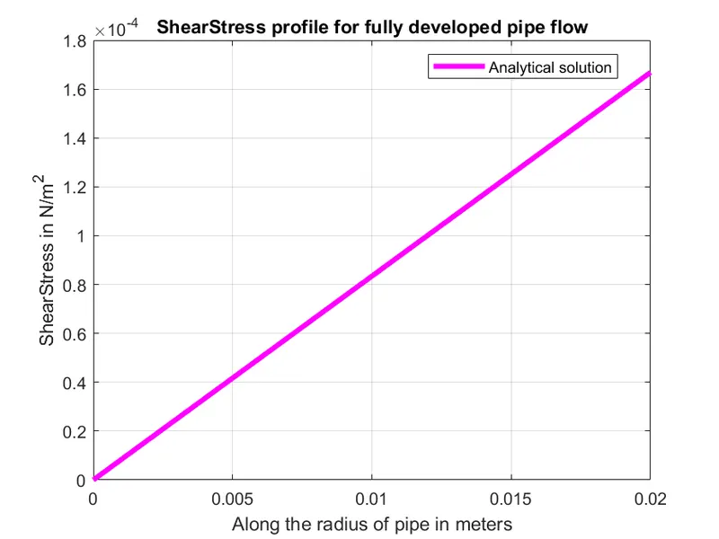
Analytical Results:-
Numerical soluions by using openFoam:
- For numerical simulation we use openFam.
Steps:-
- We need ‘0’ and ‘constant’ and ‘system’ folders in case and for runnig we need a solver.
- Firstly we setup ‘0’ and ‘constant’ and ‘system’ folders.
- In system folder we have to make block mesh dict file so that till mesh part will take care of that.
- By using matlab we create blockmesh dict file or simply we automate the process so that blockmeshdict file will come in text file formate.
- For matlab,we give inputs are diameter and length of pipe and wedge angle and renolds number and we do simulation using wedge and in this wedge we mainatin all conditions like pipe had.
- You can see the matlab code in programming section which is there at the end of the report.
- Aftrer mesh we give initial conditions which is there in ‘0’ folder.
- Here we have ‘P’ and ‘U’ are the flow field variables.
- In ‘P’ file we give kinematic pressure which we calculated using equation 6.
- In ‘U’ file we give average velocity ‘Vavg’
- Then we made blockmesh by using blockMesh command and we do simulation by help of solver.
OUTPUT:-
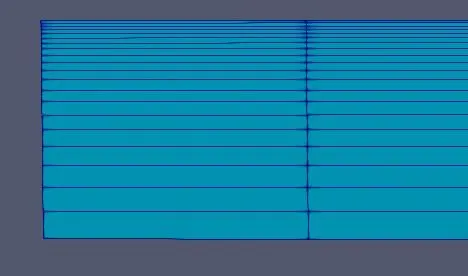
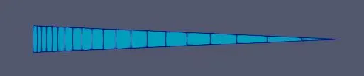
Fig(5) Mesh fornt view Fig(6) Mesh side view
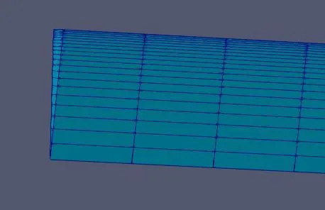
Fig(7) : Mesh isometric view
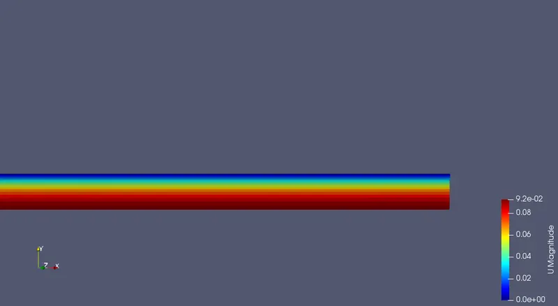
Fig(8): velocity changes at outlet and here we can observe max velocity as 0.0092 m/sec
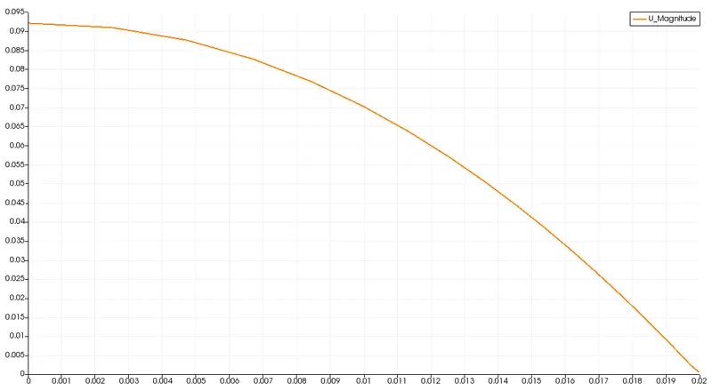
Fig(9): Velocity profile at steady state for flow through pipe numerical simulation
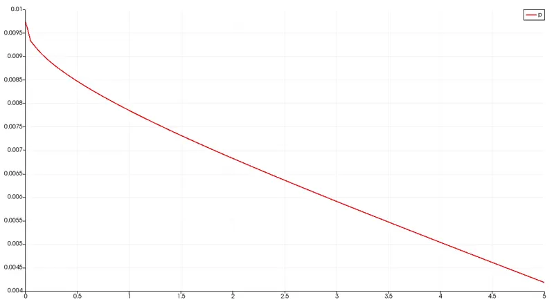
Fig(10): pressure changes at steady state for floe through pipe along the length
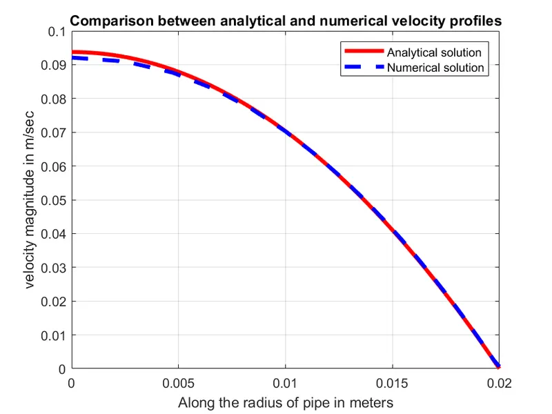
Fig(11)
Shear stress: -
- In analytical results we can see that shear stress variation with respect to radius .from that graph we can say that at steady state at mid-section of pipe we have 0 N/m2 shear stress and at the wall of the pipe maximum and constant value.
- From figure 4 and equation 2 we can say that shear stress at wall is constant and we can write it as
Γw = μ ꝺu/ ꝺr |wall
= 0.0089*(Vmax*r)/R
- At r=R we can get shear stress at wall
Γw = 1.66841536*10-4 N/m2
Conclusion: -
- From figure 11 we can say that velocity profiles at steady state nearly same.
- As we mentioned above, we attain fully developed flow after the hydrodynamic entry length. That’s why we took total length of the pipe more than the hydrodynamic entry length.
- we found maximum velocity and we got nearly same maximum value in both solutions.
- Pressure loss in laminar flows very less compare to turbulent flows. we found this pressure loss to find kinematic pressure which is helped to give input as initial boundary in numerical simulation.
MATLAB CODE for BlockMeshDict automation:-
clc;
clear all;
close all;
%% header text
h1 = '/*--------------------------------*- C++ -*----------------------------------*\';
h2 = '=========                 |';
h3 = '\\      /  F ield         | OpenFOAM: The Open Source CFD Toolbox';
h4 =  ' \\    /   O peration     | Website:  https://openfoam.org';
h5=  '\\  /    A nd           | Version:  8';
h6 = ' \\/     M anipulation  |';
h7 = '\*---------------------------------------------------------------------------*/';
h8 = 'FoamFile';
h9 = '{';
h10= 'version     2.0;';
h11 = 'format      ascii;';
h12 =  'class       dictionary;';
h13 = 'object      blockMeshDict;';
h14 ='}';
h15 = '// * * * * * * * * * * * * * * * * * * * * * * * * * * * * * * * * * * * * * //';
%% Inputs
Re = 2100;
D =0.04;
mu =0.00089;
rho =997;
Lh = 0.05*Re*D;
L =Lh+0.8;
theta = 5;
r = D/2;
%%
f1= fopen('blockMeshDict.txt','w');
fprintf(f1,'%s\n',h1);
fprintf(f1,'%s\n',h2);
fprintf(f1,'%s\n',h3);
fprintf(f1,'%s\n',h4);
fprintf(f1,'%s\n',h5);
fprintf(f1,'%s\n',h6);
fprintf(f1,'%s\n',h7);
fprintf(f1,'%s\n',h8);
fprintf(f1,'%s\n',h9);
fprintf(f1,'\t%s\n',h10);
fprintf(f1,'\t%s\n',h11);
fprintf(f1,'\t%s\n',h12);
fprintf(f1,'\t%s\n',h13);
fprintf(f1,'%s\n',h14);
fprintf(f1,'%s\n\n\n',h15);
fprintf(f1,'convertToMeters 1;\n\n');
fprintf(f1,'vertices\n');
fprintf(f1,'(\n');
fprintf(f1,'\t(%d %d %d)\n',0,0,0);
fprintf(f1,'\t(%d %f %f)\n',0,r*cosd(theta/2),r*sind(theta/2));
fprintf(f1,'\t(%d %f %f)\n',0,r*cosd(theta/2),-r*sind(theta/2));
fprintf(f1,'\t(%d %d %d)\n',L,0,0);
fprintf(f1,'\t(%d %f %f)\n',L,r*cosd(theta/2),r*sind(theta/2));
fprintf(f1,'\t(%d %f %f)\n',L,r*cosd(theta/2),-r*sind(theta/2));
fprintf(f1,');\n\n');

%%
fprintf(f1,'blocks\n\n');
fprintf(f1,'(\n\n');
fprintf(f1,'\thex (%d %d %d %d %d %d %d %d) (%d %d %d) simpleGrading (%d %d %d)\n\n',0,3,5,2,0,3,4,1,200,20,1,1,0.1,1);
fprintf(f1,');\n\n');
fprintf(f1,'edges\n');
fprintf(f1,'(\n\n');
fprintf(f1,'\tarc %d %d (%d %d %d)\n',1,2,0,r,0);
fprintf(f1,'\tarc %d %d (%d %d %d)\n\n',4,5,L,r,0);
fprintf(f1,');\n\n');
fprintf(f1,'boundary\n\n');
fprintf(f1,'(\n\n');
fprintf(f1,'\tinlet\n');
fprintf(f1,'\t{\n');
fprintf(f1,'\t\ttype patch;\n');
fprintf(f1,'\t\tfaces\n');
fprintf(f1,'\t\t(\n');
fprintf(f1,'\t\t\t(%d %d %d %d)\n',0,1,2,0);
fprintf(f1,'\t\t);\n');
fprintf(f1,'\t}\n\n');
fprintf(f1,'\toutlet\n');
fprintf(f1,'\t{\n');
fprintf(f1,'\t\ttype patch;\n');
fprintf(f1,'\t\tfaces\n');
fprintf(f1,'\t\t(\n');
fprintf(f1,'\t\t\t(%d %d %d %d)\n',3,5,4,3);
fprintf(f1,'\t\t);\n');
fprintf(f1,'\t}\n\n');
fprintf(f1,'\tfront\n');
fprintf(f1,'\t{\n');
fprintf(f1,'\t\ttype wedge;\n');
fprintf(f1,'\t\tfaces\n');
fprintf(f1,'\t\t(\n');
fprintf(f1,'\t\t\t(%d %d %d %d)\n',0,3,4,1);
fprintf(f1,'\t\t);\n');
fprintf(f1,'\t}\n');
fprintf(f1,'\tback\n');
fprintf(f1,'\t{\n');
fprintf(f1,'\t\ttype wedge;\n');
fprintf(f1,'\t\tfaces\n');
fprintf(f1,'\t\t(\n');
fprintf(f1,'\t\t\t(%d %d %d %d)\n',0,2,5,3);
fprintf(f1,'\t\t);\n');
fprintf(f1,'\t}\n');
fprintf(f1,'\taxis\n');
fprintf(f1,'\t{\n');
fprintf(f1,'\t\ttype empty;\n');
fprintf(f1,'\t\tfaces\n');
fprintf(f1,'\t\t(\n');
fprintf(f1,'\t\t\t(%d %d %d %d)\n',0,3,3,0);
fprintf(f1,'\t\t);\n');
fprintf(f1,'\t}\n');
fprintf(f1,'\ttop\n');
fprintf(f1,'\t{\n');
fprintf(f1,'\t\ttype wall;\n');
fprintf(f1,'\t\tfaces\n');
fprintf(f1,'\t\t(\n');
fprintf(f1,'\t\t\t(%d %d %d %d)\n',1,4,5,2);
fprintf(f1,'\t\t);\n');
fprintf(f1,'\t}\n');
fprintf(f1,');\n\n');
fprintf(f1,'mergePatchPairs\n');
fprintf(f1,'(\n');
fprintf(f1,');\n');
fprintf(f1,'// ************************************************************************* //');
fclose(f1);
%% Analyticl_solution
d = linspace(0,r,1000);
v_avg =(2100*(mu/rho))/D;
v_max = 2*v_avg;
v_anl = v_max*(1-((2*d./D).^2));
tau_anl = (2*mu*v_max/r).*(d);
figure(1)
plot(d,v_anl,'-m','linewidth',3);
xlabel('Along the radius of pipe in meters');
ylabel('velocity magnitude in m/sec');
title('Velocity profile for fully developed pipe flow');
legend('Analytical solution');
grid on;
%%
figure(2)
plot(d,tau_anl,'-m','linewidth',3);
xlabel('Along the radius of pipe in meters');
ylabel('ShearStress in N/m^2');
title('ShearStress profile for fully developed pipe flow');
legend('Analytical solution');
grid on;
BLOCKMESHDICT text file:-
/*--------------------------------*- C++ -*----------------------------------*\
=========                 |
\\      /  F ield         | OpenFOAM: The Open Source CFD Toolbox
 \\    /   O peration     | Website:  https://openfoam.org
\\  /    A nd           | Version:  8
 \\/     M anipulation  |
\*---------------------------------------------------------------------------*/
FoamFile
{
	version     2.0;
	format      ascii;
	class       dictionary;
	object      blockMeshDict;
}
// * * * * * * * * * * * * * * * * * * * * * * * * * * * * * * * * * * * * * //


convertToMeters 1;

vertices
(
	(0 0 0)
	(0 0.019981 0.000872)
	(0 0.019981 -0.000872)
	(5 0 0)
	(5 0.019981 0.000872)
	(5 0.019981 -0.000872)
);

blocks

(

	hex (0 3 5 2 0 3 4 1) (200 20 1) simpleGrading (1 1.000000e-01 1)

);

edges
(

	arc 1 2 (0 2.000000e-02 0)
	arc 4 5 (5 2.000000e-02 0)

);

boundary

(

	inlet
	{
		type patch;
		faces
		(
			(0 1 2 0)
		);
	}

	outlet
	{
		type patch;
		faces
		(
			(3 5 4 3)
		);
	}

	front
	{
		type wedge;
		faces
		(
			(0 3 4 1)
		);
	}
	back
	{
		type wedge;
		faces
		(
			(0 2 5 3)
		);
	}
	axis
	{
		type empty;
		faces
		(
			(0 3 3 0)
		);
	}
	top
	{
		type wall;
		faces
		(
			(1 4 5 2)
		);
	}
);

mergePatchPairs
(
);
// ************************************************************************* //
Case setup:
initial values for pressure text file:-
/*--------------------------------*- C++ -*----------------------------------*\
  =========                 |
  \\      /  F ield         | OpenFOAM: The Open Source CFD Toolbox
   \\    /   O peration     | Website:  https://openfoam.org
    \\  /    A nd           | Version:  8
     \\/     M anipulation  |
\*---------------------------------------------------------------------------*/
FoamFile
{
    version     2.0;
    format      ascii;
    class       volScalarField;
    object      p;
}
// * * * * * * * * * * * * * * * * * * * * * * * * * * * * * * * * * * * * * //

dimensions      [0 2 -2 0 0 0 0];

internalField   uniform 0;

boundaryField
{
    inlet
    {
        type            zeroGradient;
    }

    outlet
    {
        type            fixedValue;
        value       uniform 4.1835892e-3;
    }

    top
    {
        type            zeroGradient;
    }
     axis
    {
        type            empty;
    }
     front
    {
        type            wedge;
    }
     back
    {
        type            wedge;
    }
}

// ************************************************************************* //
initial values for velocity text file:-
/*--------------------------------*- C++ -*----------------------------------*\
  =========                 |
  \\      /  F ield         | OpenFOAM: The Open Source CFD Toolbox
   \\    /   O peration     | Website:  https://openfoam.org
    \\  /    A nd           | Version:  8
     \\/     M anipulation  |
\*---------------------------------------------------------------------------*/
FoamFile
{
    version     2.0;
    format      ascii;
    class       volVectorField;
    object      U;
}
// * * * * * * * * * * * * * * * * * * * * * * * * * * * * * * * * * * * * * //

dimensions      [0 1 -1 0 0 0 0];

internalField   uniform (0.0468656 0 0);

boundaryField
{
    inlet
    {
        type            fixedValue;
        value       uniform (0.0468656 0 0);

    }

    outlet
    {
        type            zeroGradient;
    }

    top
    {
        type            fixedValue;
        value       uniform (0 0 0);
    }
     axis
    {
        type            empty;
    }
     front
    {
        type            wedge;
    }
     back
    {
        type            wedge;
    }
}

// ************************************************************************* //
Transport properties:-
/*--------------------------------*- C++ -*----------------------------------*\
  =========                 |
  \\      /  F ield         | OpenFOAM: The Open Source CFD Toolbox
   \\    /   O peration     | Website:  https://openfoam.org
    \\  /    A nd           | Version:  8
     \\/     M anipulation  |
\*---------------------------------------------------------------------------*/
FoamFile
{
    version     2.0;
    format      ascii;
    class       dictionary;
    location    "constant";
    object      transportProperties;
}
// * * * * * * * * * * * * * * * * * * * * * * * * * * * * * * * * * * * * * //

nu              [0 2 -1 0 0 0 0] 8.926780341e-7;


// ************************************************************************* //
Controldict text file for time step and total time for simulation:-
/*--------------------------------*- C++ -*----------------------------------*\
  =========                 |
  \\      /  F ield         | OpenFOAM: The Open Source CFD Toolbox
   \\    /   O peration     | Website:  https://openfoam.org
    \\  /    A nd           | Version:  8
     \\/     M anipulation  |
\*---------------------------------------------------------------------------*/
FoamFile
{
    version     2.0;
    format      ascii;
    class       dictionary;
    location    "system";
    object      controlDict;
}
// * * * * * * * * * * * * * * * * * * * * * * * * * * * * * * * * * * * * * //

application     icoFoam;

startFrom       startTime;

startTime       0;

stopAt          endTime;

endTime         110;

deltaT          0.01;

writeControl    timeStep;

writeInterval   1000;

purgeWrite      0;

writeFormat     ascii;

writePrecision  6;

writeCompression off;

timeFormat      general;

timePrecision   6;

runTimeModifiable true;


// ************************************************************************* //