Week 1- Mixing Tee

Date: - 16-03-2021

Challenge 01 - Mixing Tee

Introduction: -

This type of research is very help full to get the desired temperatures by adding different temperature fluids with different velocities. This ‘T’ section application mostly we can see in air conditioners.

Domain of problem: -

Majorly, we focus on which T section will give optimum or desired outlet temperature results whether it is short or long. Which turbulence model we can use so that we can enhance the capturing of turbulence effect in simulations.

Given Inputs:-

Hot inlet temperature = 36 ^oC

Cold inlet temperature = 19 ^oC

Hot inlet velocity for both long and short mixing tee = 3 m/sec

Simulation Matrixs :-

• This simulation matrix basically tell about how many simulations we have to do

CSAE1: - short mixing tee

• Momentum ratio 2
• Momentum ratio 4

CSAE2: - Long mixing tee

• Momentum ratio 2
• Momentum ratio 4
• where momentum ration is very helpful to find out cold inlet velocity for both long and short mixing tees.
• First, we have to decide which turbulence model is helpful by using the one case and then we have to do simulations which are mentioned above.
• So, from above discussion we can conclude that we have to do 5 simulation including judgement of turbulence model.
• Finally, we have to do mech independent test by taking one case.
• Generally, we have traditional procedure which I mentioned below for CFD analysis.

Step1: Pre-processing: -

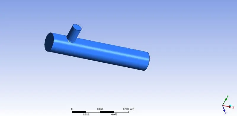
• First we took the geometry and we have to clean the body that means we need to convert mechanical body to desirable cad model.
• For this we use spacecliam to make cad model.

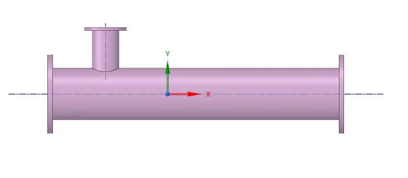
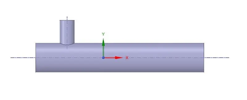
Left side is mechanical model (mixing Tee) and right side is the cad model (fluid volume of mixing Tee)

• Then next step is to create mathematical model for cad model that means meshing.
• Before mesh we give boundary conditions to body and we create mesh

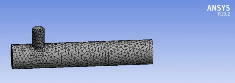
Given boundary conditions in Left side and mesh is in right side

• To get the converged results we need good quality of mesh with good quality of mesh elements.
• Here in below we can see the quality of mesh elements in mesh matric.

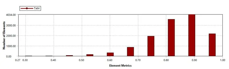
Elements quality in mesh

• Here more number of elements quality is good and all elements quality is above 30%. So we can use this mesh for further study.

Step2: solving: -

• Here for solving we used Ansys fluent.
• First we can check mesh quality and we can change units if you want. So, I changed temperature units to degree Celsius .
• In setting up physics, I gave steady state because here we are solving steady state equation and pressure based and velocity formulation is absolute.
• On the energy equation and we can choose turbulence model here.
• Important thing is the boundary conditions .
• So based on momentum ratio and velocities I gave values.
• Here I used hybrid initialization.
• In solving process we define two definitions area weighted average and standard deviation.
• Major our focus on outlet temperature after simulation so area weighted average will give temperature value at outlet .
• By having low converged standard deviation we have accurate values.

Step1: Post-processing: -

• once we completed the solving then we move to CFD post-processing to know the results.

• Here we majorly focus on temperature and velocity couture along length and cross section.
• Line plots for both temperature and velocity along length and cross section.
• We can see the results below for all cases.
• We validate our outlet temperature with analytical value for each case.

Judgment of suitable turbulence model:

• For knowing the suitable turbulence model I took first case means short mixing tee with momentum ratio 2 .
• So, hot inlet temperature is 3 m/sec and cold inlet temperature is 6 m/sec.
• Here we examine in-between k-epsilon and k-w SST turbulence models which model is best for this problem.

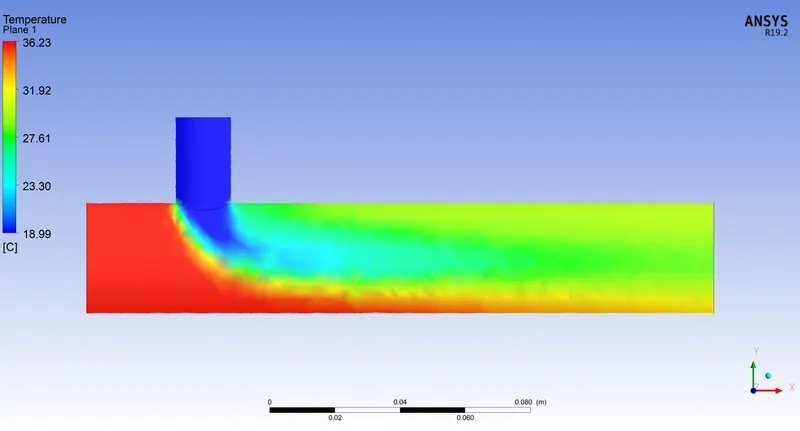
Fig(1) – Temperature couture by using K-epsilon model

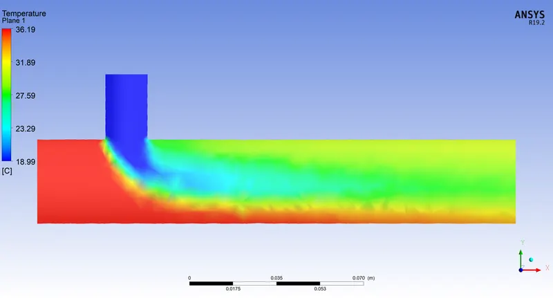
Fig(2) – Temperature couture by using K-w SST model

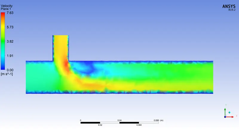
Fig(3) – Velocity couture by using K-epsilon model

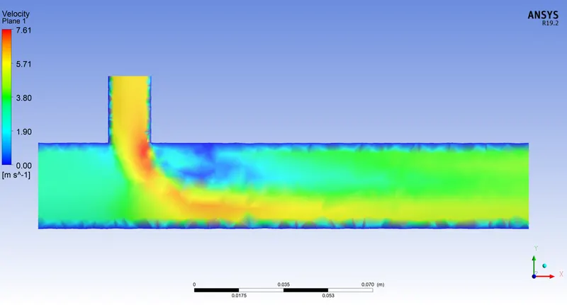
Fig(4) – Velocity couture by using K-w SST model

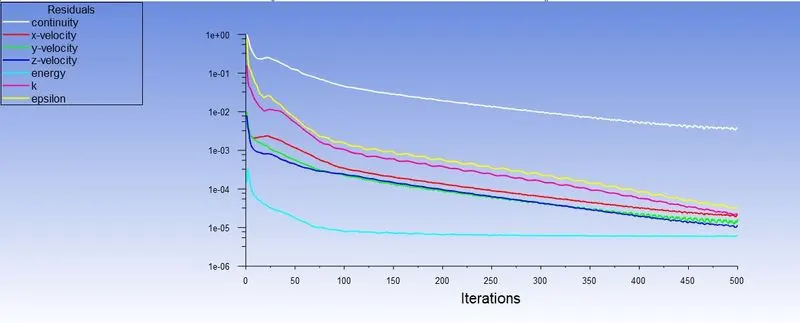
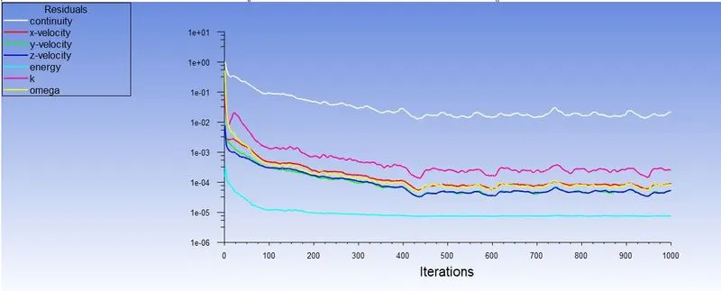
Fig (5) – Residuals of governing and transport equations of both k-epsilon and k-w SST models

Observation form above results: -

• By comparing the above couture’s we can say that K-w SST model is extracting model turbulence effect compare with k-epsilon model.
• From figure 5 we can say that for getting converge solutions k-w SST model is taking more time compare with k-epsilon model.
• Finally, we can say that we can use k-w SST turbulence model for further simulations.

Results: -

• Now we can simulate all cases with both long and short mixing Tee and end of the results we can discuss about which models is best to giving optimum outlet temperature.

Case1: - Short mixing Tee

(I) Momentum raion2: -

Fig (6) – Residuals of both governing and transport equations

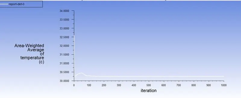
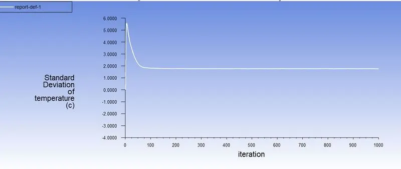
Fig (7) – Area weighted average and standard deviation for outlet mixing temperature

Fig (8) – Temperature and velocity couture along the length of Tee

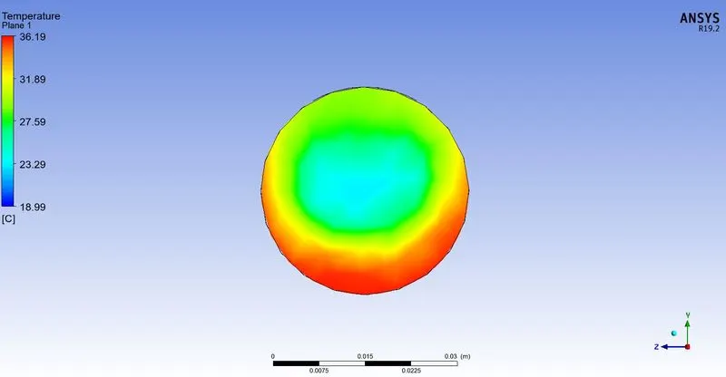
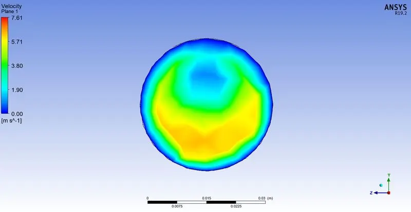
Fig (9) – Temperature and velocity couture along the cross-section of Tee

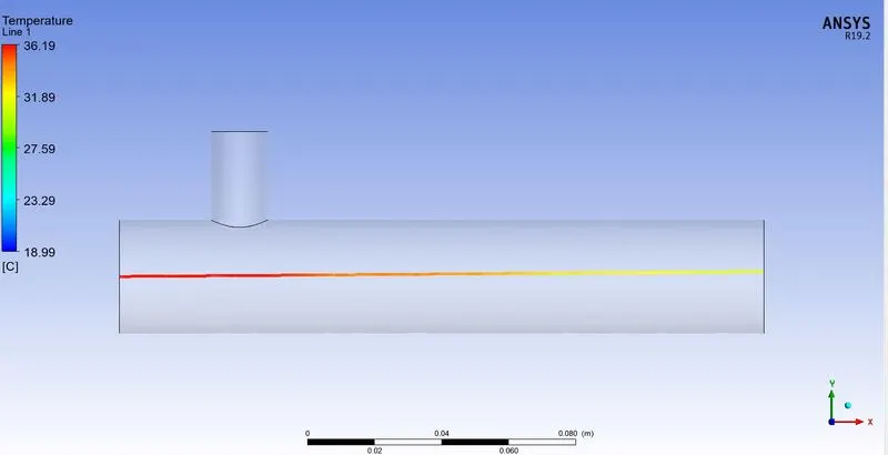
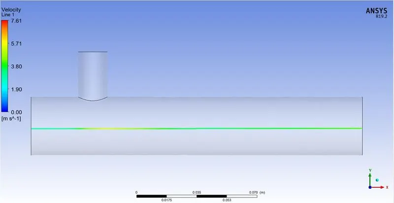
Fig (10) – Temperature and velocity line plots along the length of Tee

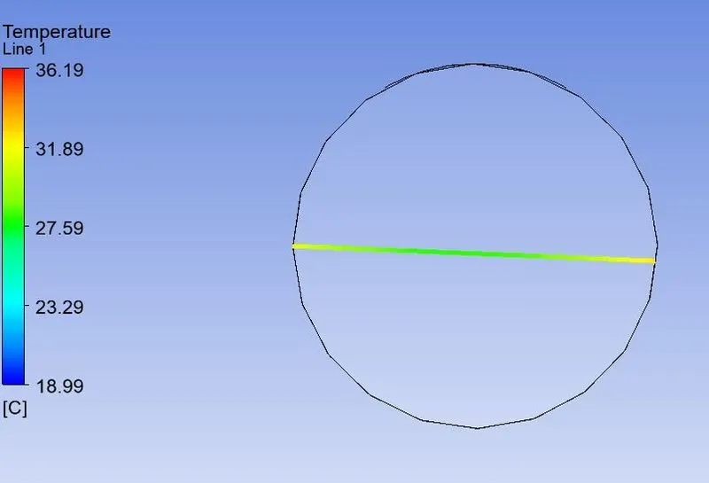
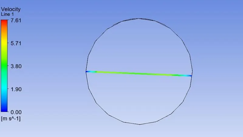
Fig (11) – Temperature and velocity line plots along the cross-section of Tee

Outlet temperature validation: -

• Numerical temperature value at outlet is 30.256 ^oC.

• Analytical formula for T_mix value at outlet is

T_mix = [(m_hot * T_hot) + (m_cold * T_cold)] / (m_hot + m_cold)

Where, m – mass flow rate = ρ * A*V

T_cold - Temperature at cold inlet = 19^oC

T_hot - Temperature at hot inlet = 36 ^oC

T_mix - outlet temperature after mixing

A_hot = 901.3138 mm², A_cold = 225.9823 mm² , V_hot = 3 m /s , V_cold = 6 m /s

T_mix = 30.322 ^oC

• By comparing both numerical and analytical solution we can say that % of difference is very less.

(II) Momentum raion4: -

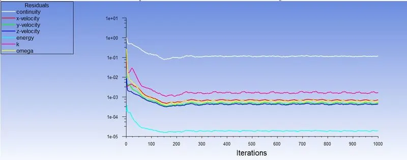
Fig (12) – Residuals of both governing and transport equations

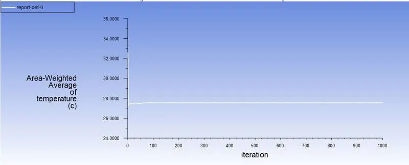
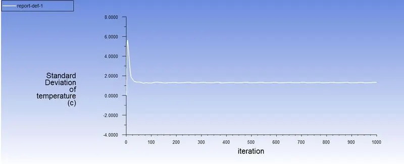
Fig (13) – Area weighted average and standard deviation for outlet mixing temperature

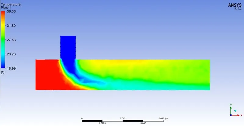
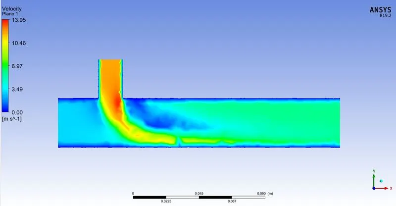
Fig (14) – Temperature and velocity couture along the length of the Tee

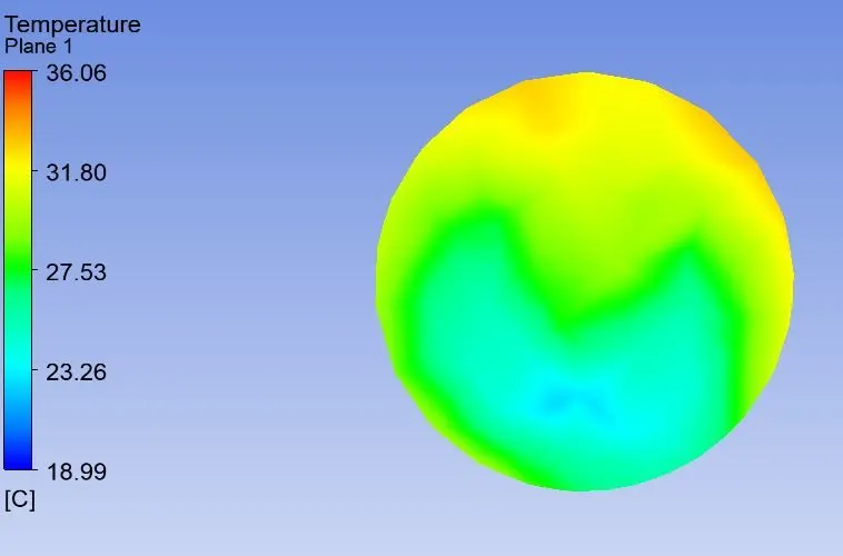
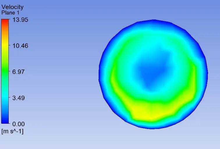
Fig (15) – Temperature and velocity couture along the cross-section of Tee

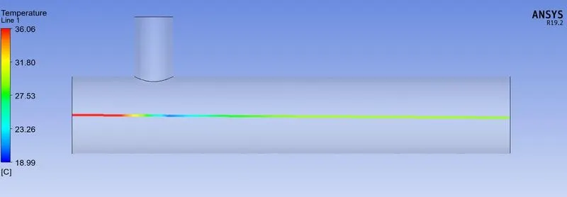
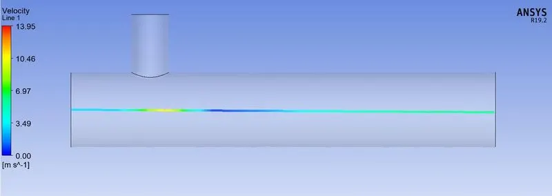
Fig (16) – Temperature and velocity line plots along the length of Tee

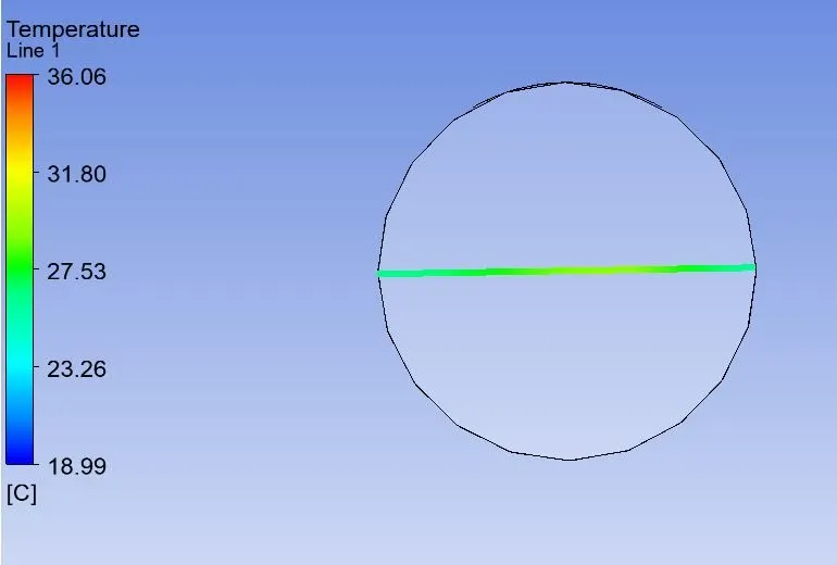
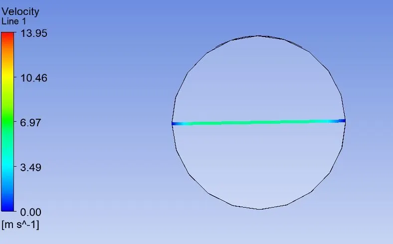
Fig (17) – Temperature and velocity line plots along the cross-section of Tee

Outlet temperature validation: -

• Numerical temperature value at outlet is 27.5371 ^oC.

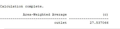
• Analytical formula for T_mix value at outlet is

T_mix = [(m_hot * T_hot) + (m_cold * T_cold)] / (m_hot + m_cold)

Where, m – mass flow rate = ρ * A*V

T_cold - Temperature at cold inlet = 19^oC

T_hot - Temperature at hot inlet = 36 ^oC

T_mix - outlet temperature after mixing

A_hot = 901.3138 mm², A_cold = 225.9823 mm² , V_hot = 3 m /s , V_cold= 12 m /s

T_mix = 27.4877^oC

• By comparing both numerical and analytical solution we can say that % of difference is very less

Case2: - Long mixing Tee

(III) Momentum raion2: -

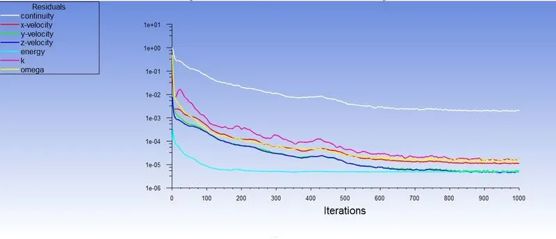
Fig (18) – Residuals of both governing and transport equations

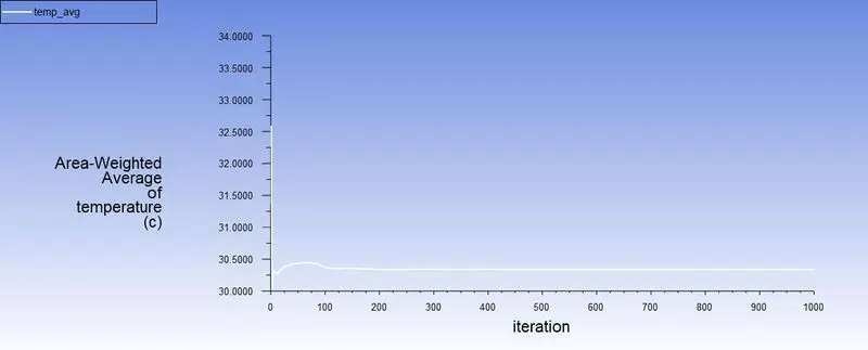
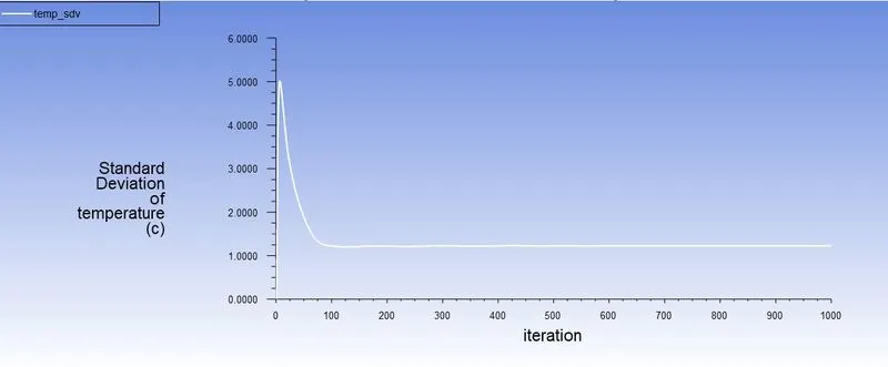
Fig (19) – Area weighted average and standard deviation for outlet mixing temperature

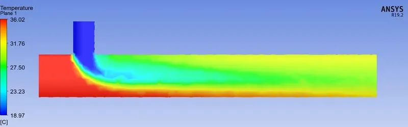
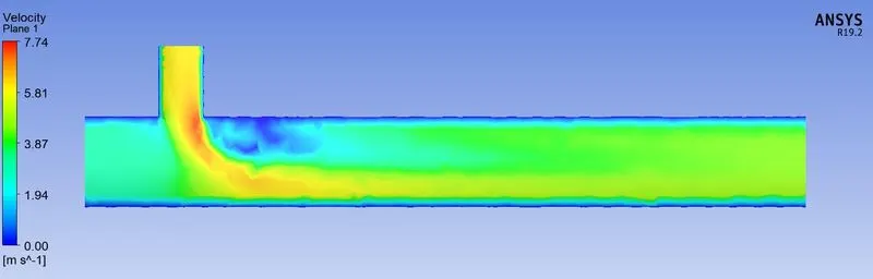
Fig (20) – Temperature and velocity couture along the length of Tee

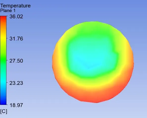
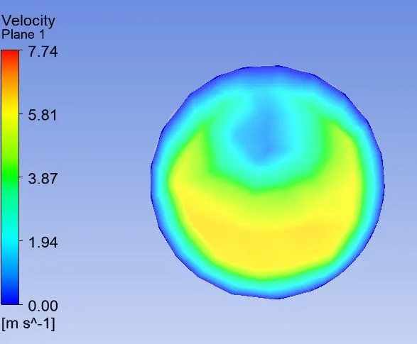
Fig (21) – Temperature and velocity couture along the cross-section of Tee

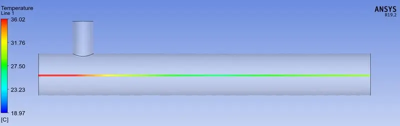
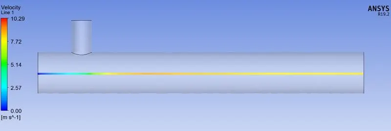
Fig (22) – Temperature and velocity line plots along the length of Tee

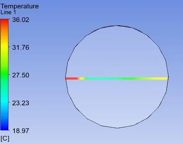
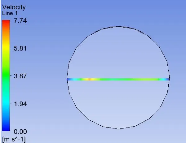
Fig (23) – Temperature and velocity line plots along the cross-section of Tee

Outlet temperature validation: -

• Numerical temperature value at outlet is 30.342^oC.

• Analytical formula for T_mix value at outlet is

T_mix = [(m_hot * T_hot) + (m_cold * T_cold)] / (m_hot + m_cold)

Where, m – mass flow rate = ρ * A*V

T_cold - Temperature at cold inlet = 19^oC

T_hot - Temperature at hot inlet = 36 ^oC

T_mix - outlet temperature after mixing

A_hot = 901.3138 mm², A_cold = 225.9823 mm² , V_hot = 3 m /s , V_cold = 6 m /s

T_mix = 30.322 ^oC

• By comparing both numerical and analytical solution we can say that % of difference is very less

(IV) Momentum raion4: -

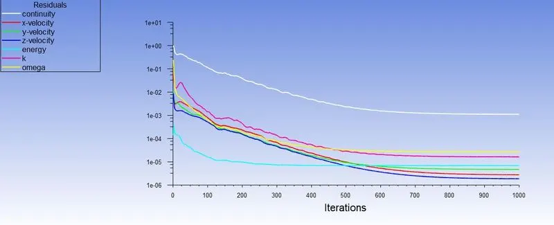
Fig (24) – Residuals of both governing and transport equations

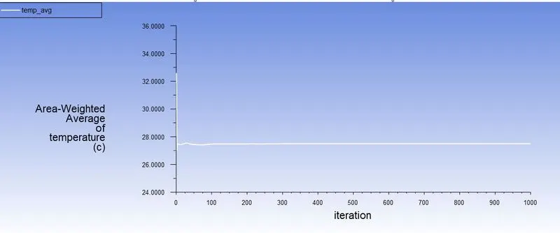
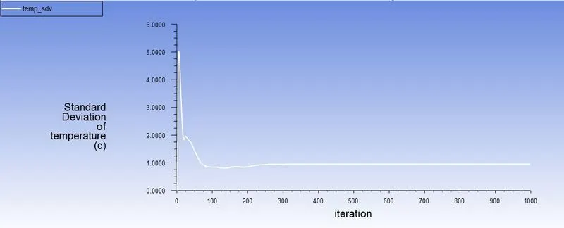
Fig (25) – Area weighted average and standard deviation for outlet mixing temperature

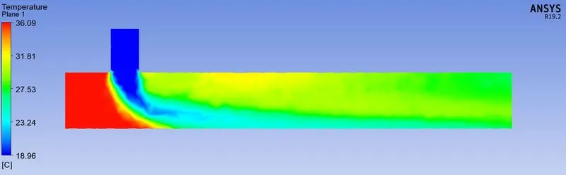
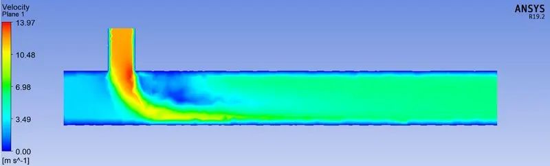
Fig (26) – Temperature and velocity couture along the length of Tee

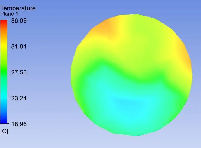
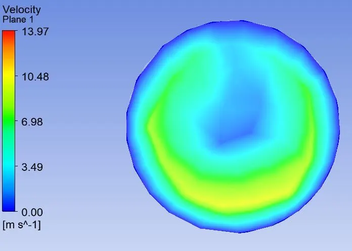
Fig (27) – Temperature and velocity couture along the cross-section of Tee

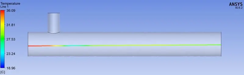
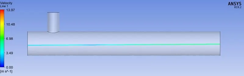
Fig (28) – Temperature and velocity line plots along the length of Tee

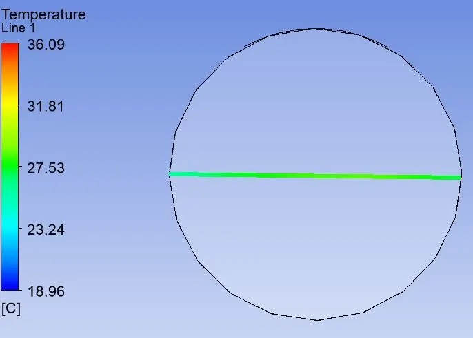
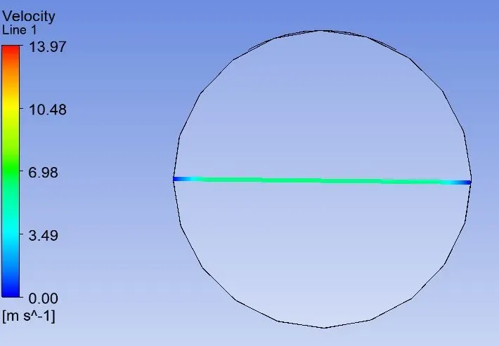
Fig (29) – Temperature and velocity line plots along the cross-section of Tee

Outlet temperature validation: -

• Numerical temperature value at outlet is 27.4915 ^oC.

• Analytical formula for T_mix value at outlet is

T_mix = [(m_hot * T_hot) + (m_cold * T_cold)] / (m_hot + m_cold)

Where, m – mass flow rate = ρ * A*V

T_cold - Temperature at cold inlet = 19^oC

T_hot - Temperature at hot inlet = 36 ^oC

T_mix - outlet temperature after mixing

A_hot = 901.3138 mm², A_cold = 225.9823 mm² , V_hot = 3 m /s , V_cold= 12 m /s

T_mix = 27.4877^oC

• By comparing both numerical and analytical solution we can say that % of difference is very less.

Comparison between two cases: -

	Momentum Ratio	No: elements	Average Outlet Temperature in Celsius	No: iterations for convergence
Short Tee	2	13014	30.2558	200
	4	13014	27.5370	210
Long Tee	2	15640	30.3419	250
	4	15640	27.4915	260

Effect of length and momentum ratio on results: -

• From above results we can say that outlet temperature is independent of length of the mixing tee.
• Momentum ratio effects the outlet temperature. By increasing the momentum ratio outlet temperature is dropping.
• From above validation of numerical and analytical values we can say that numerical simulation values are matching with analytical values.

Mesh independent study: -

• Here I took short mixing tee momentum ratio 2 case.

No: of simulations	No: elements	Average Outlet Temperature in Celsius
1	13014	30.256
2	14453	30.211
3	39951	30.272

• From above table we can say that our mesh is independent that means there is no large changes in outlet temperature by increasing the number of elements.
• So we can prefer less number of elements mesh also for simulations.
• The main advantage of this study is to decrease the computational time for solving.