Week 10: Modeling and Simulation of flow around an Ahmed Body

AIM

The aim of this validation project is to simulate and validate the flow over an Ahmed Body

OBJECTIVES

• Creating the CAD file for the Ahmed body
• Making of virtual wind tunnel for the car
• Simulating the case and validation of results with experimental values

AHMED BODY

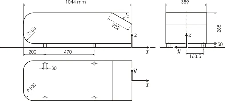
The Ahmed body was described originally by S. R. Ahmed in 1984. Three main features were seen in the wake:

1. The A recirculation region that is formed as the flow separates at the top of the vertical back surface of the model

2. The B recirculation region is formed due to the separation at the base of the model.

3. The c-pillar vortices that form as the vorticity in the side boundary layers roll up over the slant edges.

The wake was shown to be highly dependent on slant angle. For slant angles less than 12°, the flow remains attached over the slant. The flow is essentially two-dimensional and has low drag. Between 12° and 30° the flow becomes much more three-dimensional as the c-pillar vortices form. These reach maximum strength at 30°. The drag increases significantly as the low-pressure cores act on the rear surfaces. Past 30° the flow separates fully off the slant. This results in a sudden decrease in drag and weaker c-pillar vortices.

The Ahmed body (Fig. 1) was first defined and its characteristics were described in the experimental work of Ahmed. Two configurations with slant angles of 25°and 35°are considered as a test case. For these configurations detailed LDA Measurements have been performed by Becker, Lienhart, and Stoots in the LSTM low-speed wind tunnel with a cross-section of 1.87x1.4 m2 (width x height) with a bulk velocity of 40 m/s. The test section of the wind tunnel was 3/4 open (only ground plate present). The distance between the body and the plate representing the ground is 50 mm. In the experiment performed by Ahmed, flow velocity was taken 60 m/s, Reynolds number was 4.29 million based on model length.

The “Ahmed” body has the form of a highly simplified car, consisting of a blunt nose with rounded edges fixed onto a box-like middle section and a rear end that has an upper slanted surface (like a “hatch-back” car), the angle of which can be varied. The model is supported on circular-sectioned legs or stilts, rather than wheels. Despite neglecting a number of features of a real car (rotating wheels, rough underside, surface projections, etc.) the Ahmed body generates the essential features of flow around a car, namely: flow impingement and displacement around the nose, relatively uniform flow around the middle and flow separation and wake generation at the rear. Studying such a simplified car body aims to understand the flow processes involved in drag production. By understanding the mechanisms involved in generating drag, one should design a car to minimize drag and, therefore, minimize fuel consumption and maximize performance. The principal contribution to drag experienced by a car is pressure drag. The rear of the vehicle provides a major contribution to pressure drag. In particular, the rear slant angle is critical in determining the mode of the wake flow and hence the drag experienced by the vehicle. Janssen & Hucho found that the maximum drag was obtained for a vehicle with rear slant angle β ≈ 30◦ (to the horizontal) where the flow over the slant remained partially attached and longitudinal trailing vortices were formed at the edges of the slant. For steeper slant angles (β > 30◦ ) the flow over the rear slant became fully separated and the drag decreased.

SIMULATION

Geometry

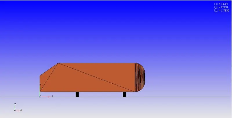
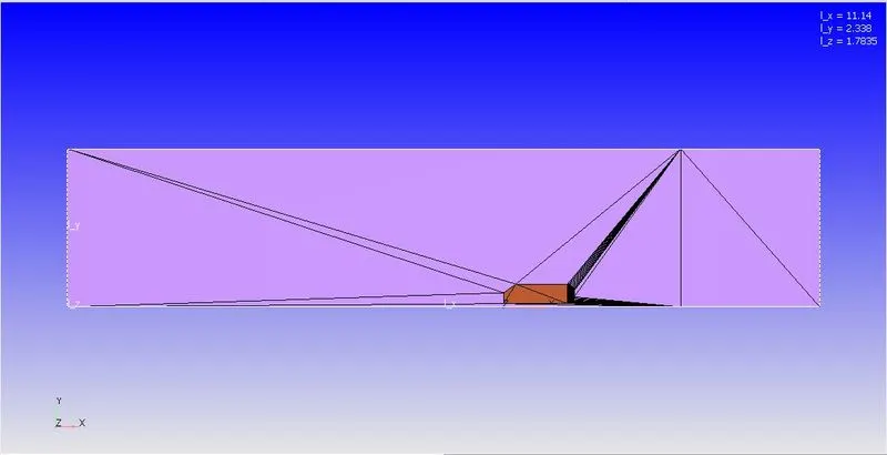
The geometry file was created in a CAD package and imported into the Converge CFD. The virtual wind tunnel was created according to some assumed dimensions. The dimensions of the wind tunnel are displayed on the right side of the image.

Setup

The setup of the simulation is as follows

1. Species - Air
2. Solver - Transient
3. Start Time - 0 s
4. End Time - 0.2 s
5. Turbulence Model - K - Omega SST
6. Base Grid = 0.09m
7. Fixed Embedding - Box
8. Scale - 2
9. Boundary Conditions

Inlet

1. Inlet - Inflow BC
2. Velocity = 40 m/s
3. Temperature = 300 K
4. Species - Air

Outlet

1. Outlet - Outflow BC
2. Pressure = 101325 Pa
3. Temperature = 300 K
4. Species - Air

Ahmed Body

1. Law of wall BC
2. Temperature = 300 K

No-Slip wall

1. No-Slip BC
2. Temperature = 300 K

Symmetry Wall

1. Symmetry BC

Results

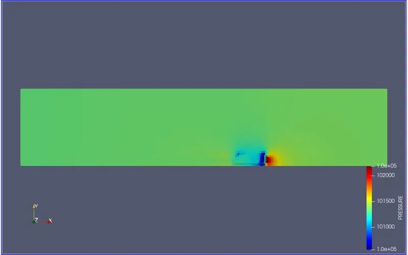
Pressure Contour

Velocity Contour

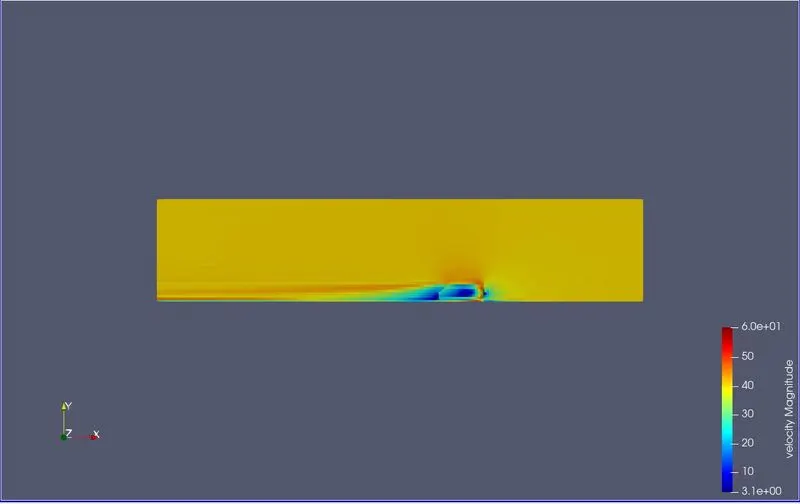
The 3d Geometry was cut in half. From the contours, we see that the wake region has not been accurately captured accurately cause of the limitations of the computational power available in the laptop. The low-pressure regions are the main reason for the formation of the recirculation zone which leads to the wake region.

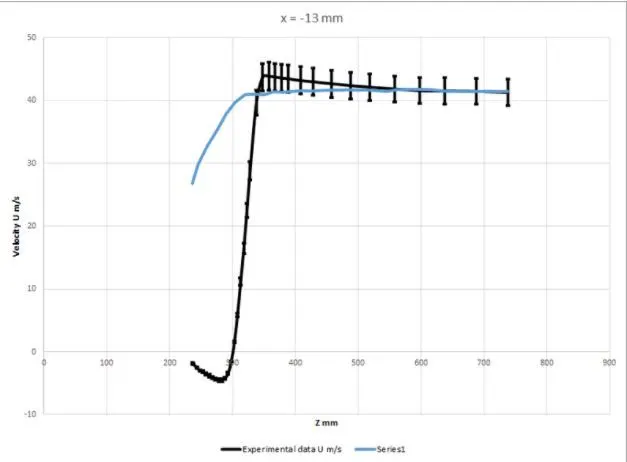
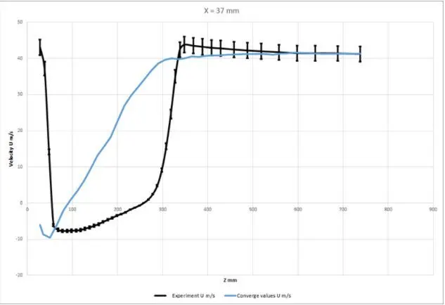
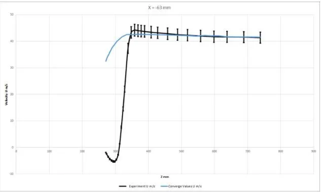
VELOCITY COMPARISON OF SIMULATION AND EXPERIMENTAL DATA

VELOCITY PLOT AT X = -13 mm

VELOCITY PLOT AT X = 37 mm

VELOCITY PLOT AT X = -63 mm

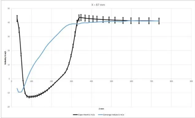
VELOCITY PLOT AT X = 87 mm

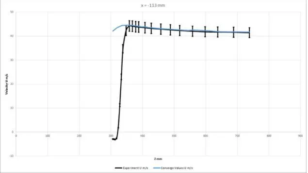
VELOCITY PLOT AT X = -113 mm

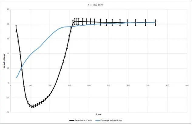
VELOCITY PLOT AT X = 187 mm

For the comparison of the simulation and experimental data,

1. we first have to locate the center of the geometry in ParaView.
2. Next, we create the line probes at the respective x locations
3. The data of the velocity is then exported to an excel sheet from the paraview
4. Using the line plot command we create the plot for the simulation curve (Blue Colour)
5. Experimental Data was downloaded from the source provided to us which contains the x velocity data
6. The black curve shows the experimental data.
7. The accepted error percentage is 5% in general industrial purposes, as I was low on computational power which is needed to run the simulation.
8. The error percentage bar already shows initially they are in a good match but as the mesh moves away the error starts to build.

NORMALISED DATA

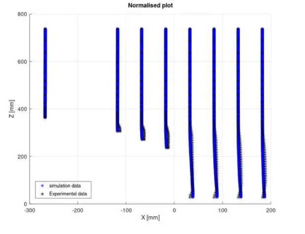
This plot was created by feeding the values of experimental and simulation data and plotted in OCTAVE

DRAG AND LIFT FORCE

Drag Force Plot

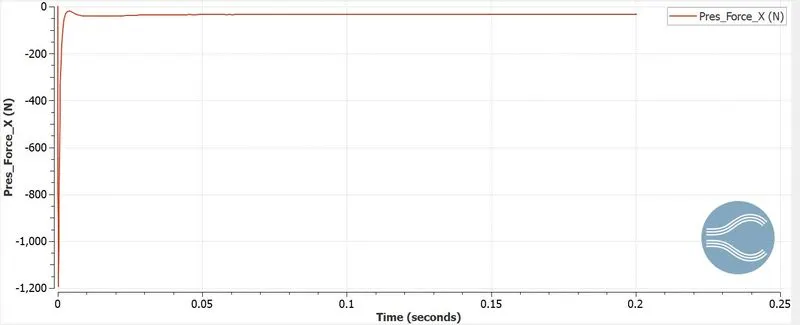
The coefficient of drag is computed from the following formula.

`F_d = 1/2*C_d*rho*A*V^2`

From the above equation, plug in the values and we get

1. F = 32.42 N
2. rho = 1.225 kg/m^3
3. A = 0.11 m^2
4. V = 40 m/s

`C_d = 0.3`

Lift Force

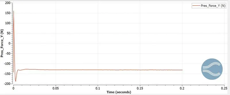
The coefficient of lift is computed from the following formula.

`F_l = 1/2C_l*rho*A*V^2`

From the above equation, plug in the values and we get

1. F = 131.74 N
2. rho = 1.225 kg/m^3
3. A = 0.11 m^2
4. V = 40 m/s

`C_l=1.22`

VELOCITY ANIMATION

PRESSURE ANIMATION

CONCLUSION

1. Experimental and simulation data was successfully validated with some increase the error due to computational Power
2. Pressure and velocity contours help to visualize the air movement over the body
3. Aerodynamic fundamentals were applied to analyze forces acting on the body