Flow over an NACA 2412 Airfoil
AIM
The aim of this project is to simulate the flow over a NACA 2412 Airfoil
OBJECTIVES
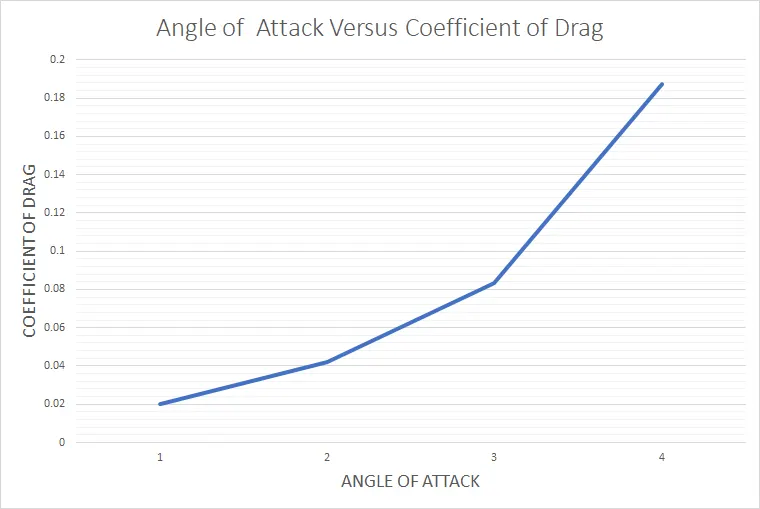
- Plot Coefficient of drag vs angle of attack
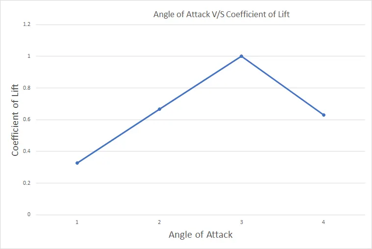
- Plot Lift Coefficient vs angle of attack
- Comparison of turbulence model results
AIRFOIL
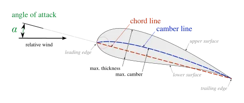
An airfoil (American English) or aerofoil (British English) is the cross-sectional shape of an object whose motion through a gas is capable of generating significant lift, such as a wing, a sail, or the blades of a propeller, rotor, or turbine. A solid body moving through a fluid produces an aerodynamic force. The component of this force perpendicular to the relative freestream velocity is called lift. The component parallel to the relative freestream velocity is called drag. An airfoil is a streamlined shape that is capable of generating significantly more lift than drag.[1] Airfoils designed for use at different speeds differ in their geometry: those for subsonic flight generally have a rounded leading edge, while those designed for supersonic flight tend to be slimmer with a sharp leading edge. All have a sharp trailing edge. Foils of similar function designed with water as the working fluid are called hydrofoils.
The lift on an airfoil is primarily the result of its angle of attack. When oriented at a suitable angle, the airfoil deflects the oncoming air (for fixed-wing aircraft, a downward force), resulting in a force on the airfoil in the direction opposite to the deflection. This force is known as aerodynamic force and can be resolved into two components: lift and drag. Most foil shapes require a positive angle of attack to generate lift, but cambered airfoils can generate lift at a zero angles of attack. This "turning" of the air in the vicinity of the airfoil creates curved streamlines, resulting in lower pressure on one side and higher pressure on the other. This pressure difference is accompanied by a velocity difference, via Bernoulli's principle, so the resulting flowfield about the airfoil has a higher average velocity on the upper surface than on the lower surface. In some situations (e.g. inviscid potential flow) the lift force can be related directly to the average top/bottom velocity difference without computing the pressure by using the concept of circulation and the Kutta–Joukowski theorem.
The various terms related to airfoils are defined below:
- The suction surface (a.k.a. upper surface) is generally associated with higher velocity and lower static pressure.
- The pressure surface (a.k.a. lower surface) has a comparatively higher static pressure than the suction surface. The pressure gradient between these two surfaces contributes to the lift force generated for a given airfoil.
The geometry of the airfoil is described with a variety of terms :
- The leading edge is the point at the front of the airfoil that has maximum curvature (minimum radius).
- The trailing edge is defined similarly as the point of maximum curvature at the rear of the airfoil.
- The chord line is the straight line connecting leading and trailing edges. The chord length, or simply chord, {displaystyle c}
 , is the length of the chord line. That is the reference dimension of the airfoil section.
The shape of the airfoil is defined using the following geometrical parameters:
- The mean camber line or mean line is the locus of points midway between the upper and lower surfaces. Its shape depends on the thickness distribution along the chord;
- The thickness of an airfoil varies along the chord. It may be measured in either of two ways:
- Thickness measured perpendicular to the camber line.This is sometimes described as the "American convention";
- Thickness measured perpendicular to the chord line. This is sometimes described as the "British convention".
Some important parameters to describe an airfoil's shape are its camber and its thickness. For example, an airfoil of the NACA 4-digit series such as the NACA 2415 (to be read as 2 – 4 – 15) describes an airfoil with a camber of 0.02 chord located at 0.40 chord, with 0.15 chord of maximum thickness.
Finally, important concepts used to describe the airfoil's behavior when moving through a fluid are:
- The aerodynamic center, which is the chord-wise length about which the pitching moment is independent of the lift coefficient and the angle of attack.
- The center of pressure, which is the chord-wise location about which the pitching moment is zero.
NACA 4 digit airfoil specification
This NACA airfoil series is controlled by 4 digits e.g. NACA 2412, which designate the camber, position of the maximum camber and thickness. If an airfoil number is
e.g.
NACA 2412
then:
- M is the maximum camber divided by 100. In the example M=2 so the camber is 0.02 or 2% of the chord
- P is the position of the maximum camber divided by 10. In the example P=4 so the maximum camber is at 0.4 or 40% of the chord.
- XX is the thickness divided by 100. In the example XX=12 so the thiickness is 0.12 or 12% of the chord.
NACA 4 digit airfoil calculation
The NACA airfoil section is created from a camber line and a thickness distribution plotted perpendicular to the camber line.
The equation for the camber line is split into sections either side of the point of maximum camber position (P). In order to calculate the position of the final airfoil envelope later the gradient of the camber line is also required. The equations are:
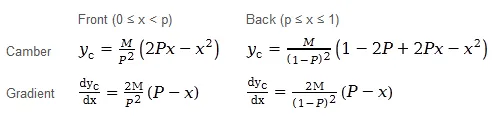
The thickness distribution is given by the equation:

- The constants a0 to a4 are for a 20% thick airfoil. The expression T/0.2 adjusts the constants to the required thickness.
- At the trailing edge (x=1) there is a finite thickness of 0.0021 chord width for a 20% airfoil. If a closed trailing edge is required the value of a4 can be adjusted.
- The value of yt is a half thickness and needs to be applied both sides of the camber line.
Using the equations above, for a given value of x it is possible to calculate the camber line position Yc, the gradient of the camber line and the thickness. The position of the upper and lower surface can then be calculated perpendicular to the camber line.
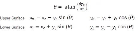
The most obvious way to to plot the airfoil is to iterate through equally spaced values of x calclating the upper and lower surface coordinates. While this works, the points are more widely spaced around the leading edge where the curvature is greatest and flat sections can be seen on the plots. To group the points at the ends of the airfoil sections a cosine spacing is used with uniform increments of β

AIRFOIL SIMULATION 1AOA
Geometry
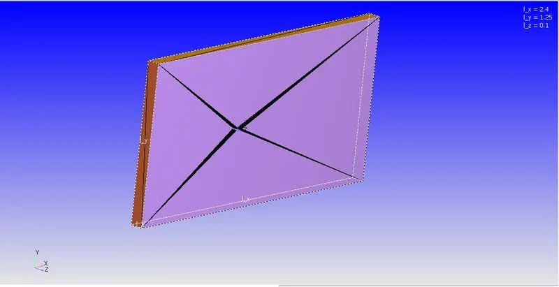
The geometry was modeled on converge studio by creating vertices and patching them using a patch tool. The wind tunnel was constructed by assuming some dimensions of the wind tunnel to be based on the chord length of the airfoil (0.1m)
Length = 2.4m (50 times chord length)
Width = 1.25m (30 times chord length)
Inlet velocity was determined by aassuming values of air as
Reynolds Number = 200000
Density of air = 1.225 `[kg]/[m^3]`
Dynamic viscosity = 1.81x10⁻⁵ `[N-s]/m^2`
From the Reynolds number equation the inlet velocity was computed to be around 30 m/s
Mesh
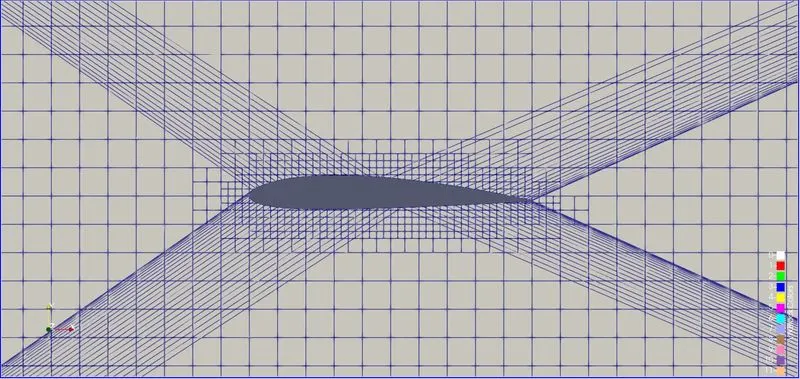
The mesh was generated with a base size of 0.01m with a fixed embedding around the airfoil to capture the effect of angle of attack on velocity and pressure contours.
Setup
- Material - Air
- Species - N2 and O2
- Solver - Transcient
- Start Time - 0 sec
- End time - 0.5 Sec
- Turbulence Model - K - Epsilon RNG
- Mesh Size = 0.01m
- boundary Conditions
Inlet
- Inlet - Inflow
- Velocity = 30 m/s
- Temperature = 300K
Outlet
- Outlet - Outflow
- Pressure = 101325 Pa
- Temperature = 300K
Top and Bottom
- Symmetry BC
Front and Back
- 2D Boundaries
Wall
- Law of Wall BC
- Temperature = 300K
- Wall - Wall BC
Results
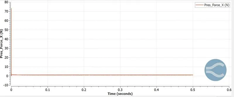
Drag Force Plot
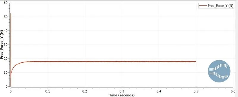
Lift Force Plot
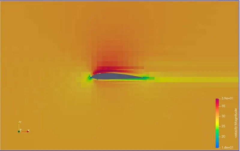
Velocity Contour
Pressure Contour
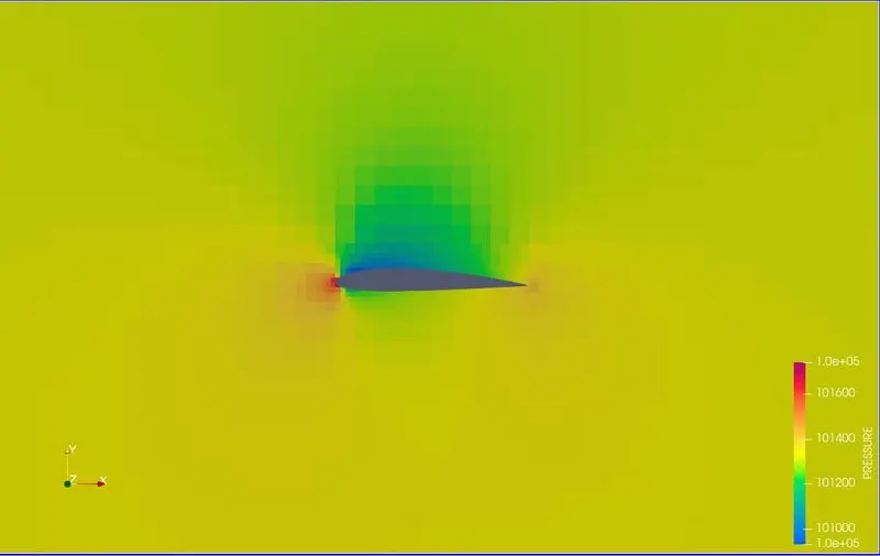
AIRFOIL SIMULATION 5AOA
Geometry
The geometry was modeled on converge studio by creating vertices and patching them using a patch tool. The wind tunnel was constructed by assuming some dimensions of the wind tunnel to be based on the chord length of the airfoil (0.1m)
Length = 2.4m (50 times chord length)
Width = 1.25m (30 times chord length)
Inlet velocity was determined by aassuming values of air as
Reynolds Number = 200000
Density of air = 1.225 `[kg]/[m^3]`
Dynamic viscosity = 1.81x10⁻⁵ `[N-s]/m^2`
From the Reynolds number equation the inlet velocity was computed to be around 30 m/s
Mesh
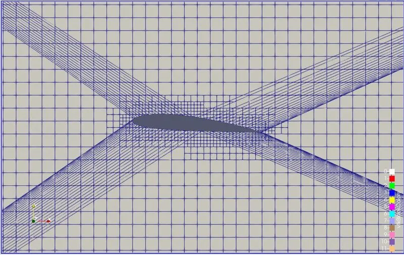
The mesh was generated with a base size of 0.01m with a fixed embedding around the airfoil to capture the effect of angle of attack on velocity and pressure contours.
Setup
- Material - Air
- Species - N2 and O2
- Solver - Transcient
- Start Time - 0 sec
- End time - 0.5 Sec
- Turbulence Model - K - Epsilon RNG
- Mesh Size = 0.01m
- boundary Conditions
Inlet
- Inlet - Inflow
- Velocity = 30 m/s
- Temperature = 300K
Outlet
- Outlet - Outflow
- Pressure = 101325 Pa
- Temperature = 300K
Top and Bottom
- Symmetry BC
Front and Back
- 2D Boundaries
Wall
- Law of Wall BC
- Temperature = 300K
- Wall - Wall BC
Results
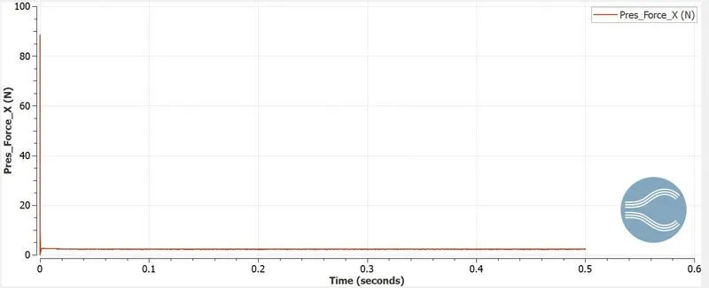
Drag Force Plot
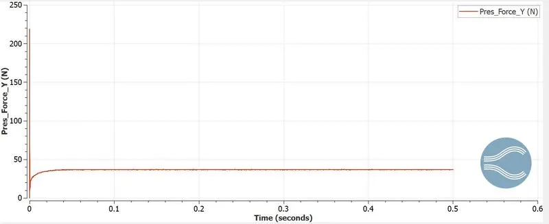
Lift Force Plot
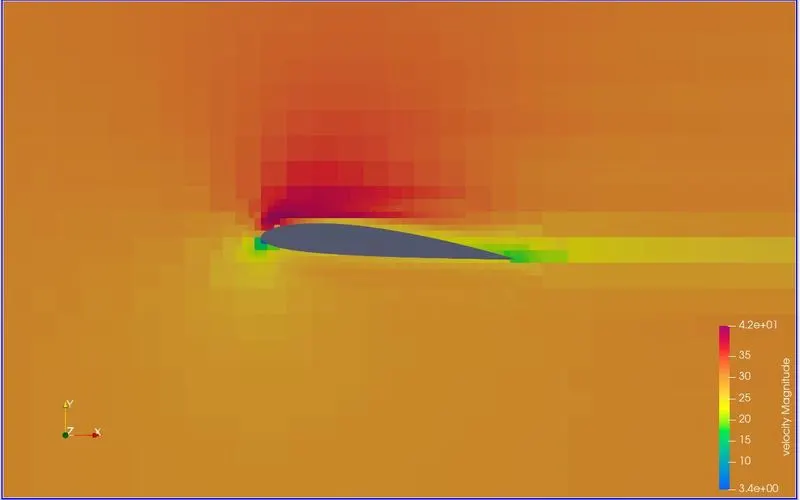
Velocity Contour
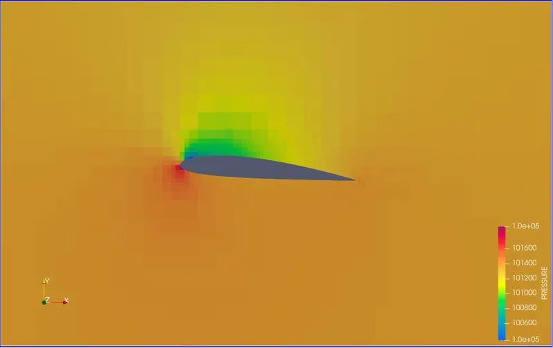
Pressure Contour
AIRFOIL SIMULATION 10AOA
Geometry
The geometry was modeled on converge studio by creating vertices and patching them using a patch tool. The wind tunnel was constructed by assuming some dimensions of the wind tunnel to be based on the chord length of the airfoil (0.1m)
Length = 2.4m (50 times chord length)
Width = 1.25m (30 times chord length)
Inlet velocity was determined by aassuming values of air as
Reynolds Number = 200000
Density of air = 1.225 `[kg]/[m^3]`
Dynamic viscosity = 1.81x10⁻⁵ `[N-s]/m^2`
From the Reynolds number equation the inlet velocity was computed to be around 30 m/s
Mesh
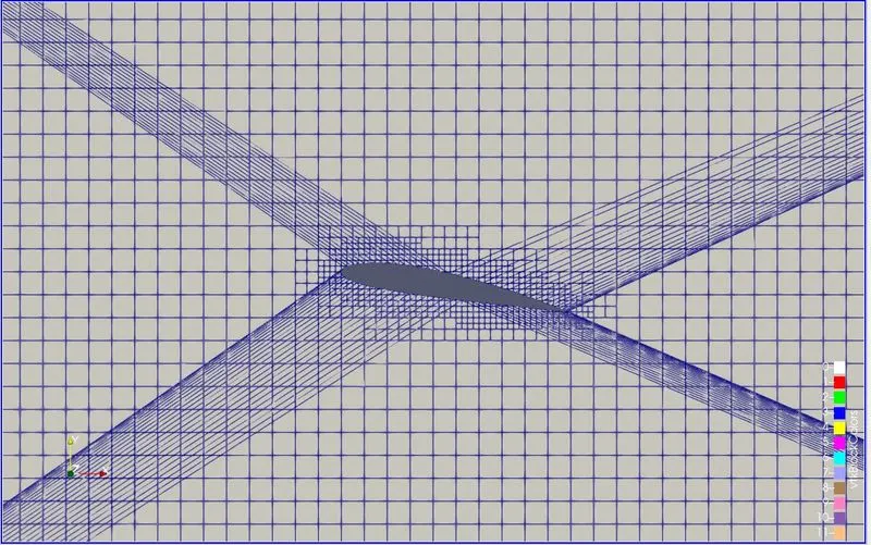
The mesh was generated with a base size of 0.01m with a fixed embedding around the airfoil to capture the effect of angle of attack on velocity and pressure contours.
Setup
- Material - Air
- Species - N2 and O2
- Solver - Transcient
- Start Time - 0 sec
- End time - 0.5 Sec
- Turbulence Model - K - Epsilon RNG
- Mesh Size = 0.01m
- boundary Conditions
Inlet
- Inlet - Inflow
- Pressure = 101325 Pa
- Temperature = 300K
Outlet
- Outlet - Outflow
- Velocity = 30 m/s
- Temperature = 300K
Top and Bottom
- Symmetry BC
Front and Back
- 2D Boundaries
Wall
- Law of Wall BC
- Temperature = 300K
- Wall - Wall BC
Results
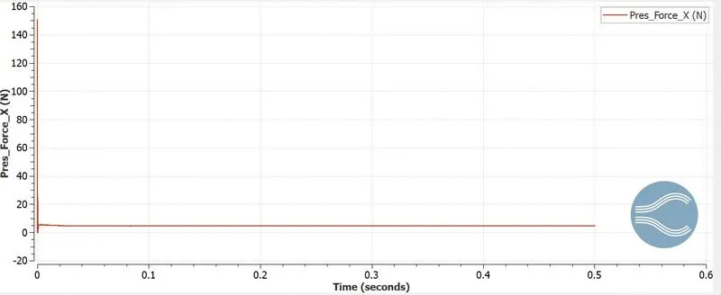
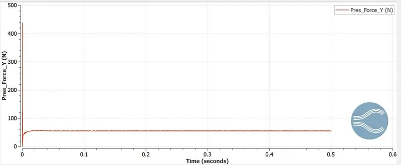
Drag Force Plot
Lift Force Plot
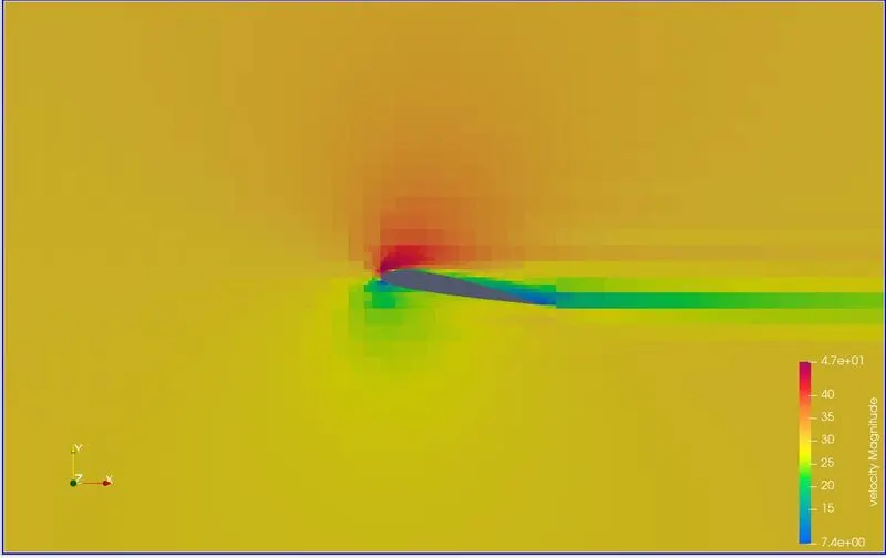
Velocity Contour
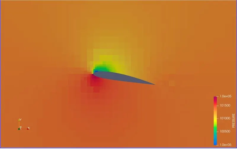
Pressure Contour
AIRFOIL SIMULATION 1AOA
Geometry
The geometry was modeled on converge studio by creating vertices and patching them using a patch tool. The wind tunnel was constructed by assuming some dimensions of the wind tunnel to be based on the chord length of the airfoil (0.1m)
Length = 2.4m (50 times chord length)
Width = 1.25m (30 times chord length)
Inlet velocity was determined by aassuming values of air as
Reynolds Number = 200000
Density of air = 1.225 `[kg]/[m^3]`
Dynamic viscosity = 1.81x10⁻⁵ `[N-s]/m^2`
From the Reynolds number equation the inlet velocity was computed to be around 30 m/s
Mesh
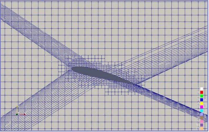
The mesh was generated with a base size of 0.01m with a fixed embedding around the airfoil to capture the effect of angle of attack on velocity and pressure contours.
Setup
- Material - Air
- Species - N2 and O2
- Solver - Transcient
- Start Time - 0 sec
- End time - 0.5 Sec
- Turbulence Model - K - Epsilon RNG
- Mesh Size = 0.01m
- boundary Conditions
Inlet
- Inlet - Inflow
- Velocity = 30 m/s
- Temperature = 300K
Outlet
- Outlet - Outflow
- Pressure = 101325 Pa
- Temperature = 300K
Top and Bottom
- Symmetry BC
Front and Back
- 2D Boundaries
Wall
- Law of Wall BC
- Temperature = 300K
- Wall - Wall BC
Results
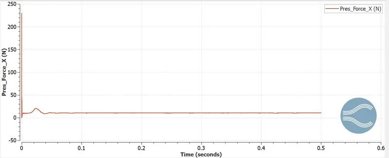
Drag Force Plot
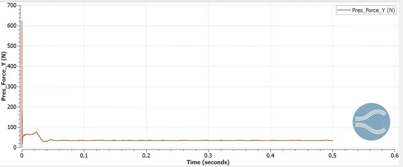
Lift Force Plot
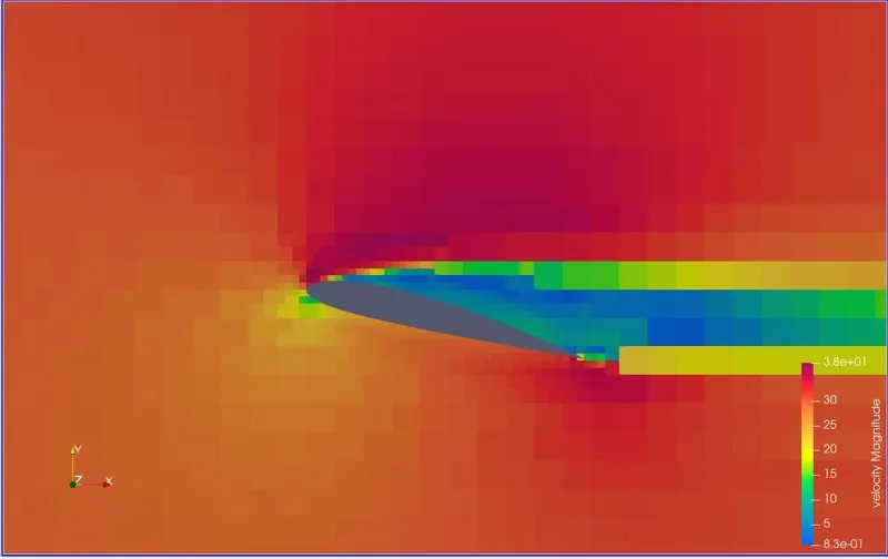
Velocity Contour
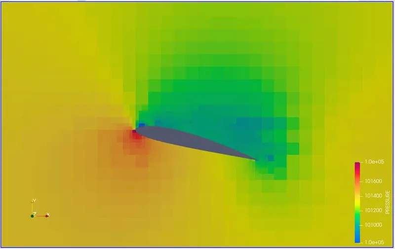
Pressure Contour
DRAG FORCE
In fluid dynamics, drag (sometimes called air resistance, a type of friction, or fluid resistance, another type of friction or fluid friction) is a force acting opposite to the relative motion of any object moving with respect to a surrounding fluid. This can exist between two fluid layers (or surfaces) or a fluid and a solid surface. Unlike other resistive forces, such as dry friction, which are nearly independent of velocity, drag force depends on velocity.
Drag force is proportional to the velocity for low-speed flow and the squared velocity for high speed flow, where the distinction between low and high speed is measured by the Reynolds number. Even though the ultimate cause of a drag is viscous friction, the turbulent drag is independent of viscosity
Drag depends on the properties of the fluid and on the size, shape, and speed of the object. One way to express this is by means of the drag equation:

where
- is the drag force,
- is the density of the fluid,
- is the speed of the object relative to the fluid,
- is the cross sectional area, and
- is the drag coefficient – a dimensionless number.
The drag coefficient depends on the shape of the object and on the Reynolds number

where
D is some characteristic diameter or linear dimension. Actually D it is the equivalent diameter
LIFT FORCE
A fluid flowing around the surface of an object exerts a force on it. Lift is the component of this force that is perpendicular to the oncoming flow direction.It contrasts with the drag force, which is the component of the force parallel to the flow direction. Lift conventionally acts in an upward direction in order to counter the force of gravity, but it can act in any direction at right angles to the flow.
he lift coefficient (CL) is a dimensionless coefficient that relates the lift generated by a lifting body to the fluid density around the body, the fluid velocity and an associated reference area. A lifting body is a foil or a complete foil-bearing body such as a fixed-wing aircraft. CL is a function of the angle of the body to the flow, its Reynolds number and its Mach number. The section lift coefficient cl refers to the dynamic lift characteristics of a two-dimensional foil section, with the reference area replaced by the foil chord
The lift coefficient CL is defined by
 ,
,
where L is the lift force, S is the relevant surface area and Q is the fluid dynamic pressure, in turn linked to the `rho`, and to the flow speed u
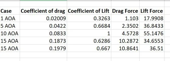
SUMMARY TABLE
Angle of Attack Versus Coefficient of Drag
Angle of Attack V/S Coefficient of Lift
CONCLUSION
- The simulation was performed on different angle of attack
- As the angle of attack increases, coefficient of drag increases
- Lift coefficient suddenly begins to drop
- Angle of attack versus drag and lift are plotted
- Aerodynamics of airfoil were analysed