Project 2 - Rankine cycle Simulator

1. AIM: -

Create a Rankine Cycle Simulator using MATLAB.

2. OBJECTIVE: -

• Calculate the state points of the Rankine Cycle based on user inputs.
• Plot the corresponding T-s and h-s plots for the given set of inputs.
• Calculate Net work output and Back work ratio

3. DESCRIPTION: -

3.1 Ideal Rankine Cycle

The Rankine cycle system consists of a pump, boiler, turbine, and condenser. The pump delivers liquid water to the boiler. The boiler heated water with the help of furnace converts water to superheated steam. This steam is used to run the turbine which powers the generator. Steam leaves the turbine and becomes cooled to liquid state in the condenser. Then the liquid is pressurized by the pump and goes back to the boiler. And the cycle continues. The figure as follow,

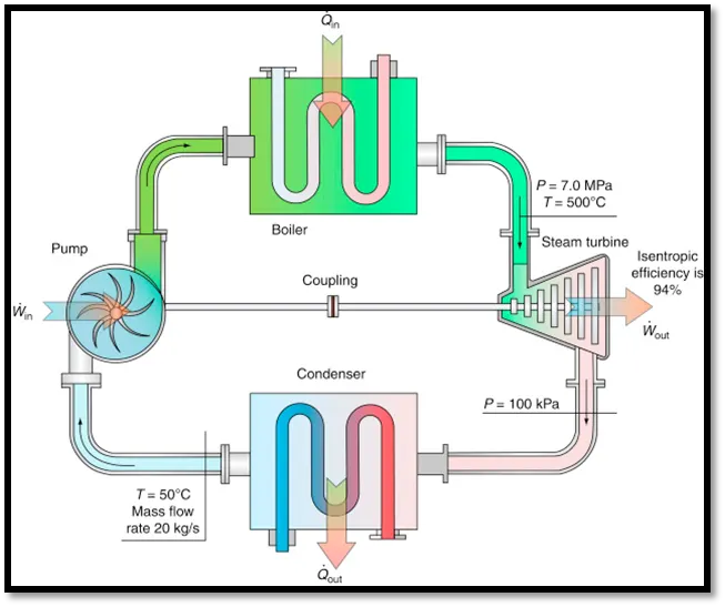
In an ideal Rankine cycle, all the units operate with the steady-state flow, and the kinetic and potential energy of the fluid are considered to be negligible compared to the temperature and pressure effects.The Rankine cycle efficiency is much higher than Carnot cycle efficiency as because the pump is used in the Rankine cycle, which gives higher work ratio by doing significant proportion of turbine work.

• Working Principle: -

Temperature(T) vs Entropy(S) diagram

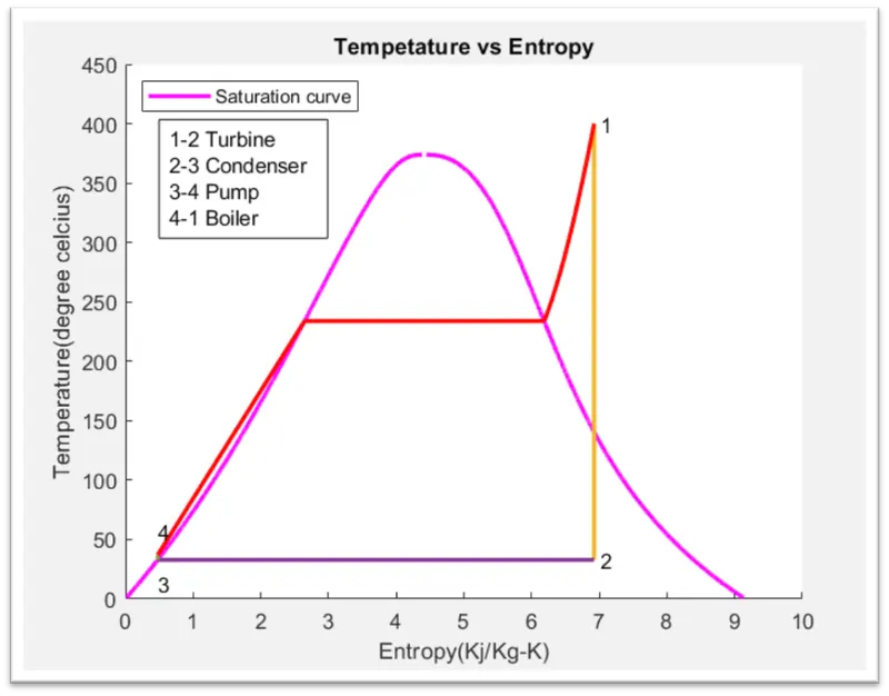
Note: -we are change the state point only as per challenge otherwise whole process is same.

The Rankine cycle is an ideal cycle if water passes through the four components without irreversibility and pressure drops. The ideal Rankine cycle consists of the following four processes: -

• State 1-2: - Isentropic or Reversible Adiabatic Expansion (Turbine)

The process 1-2 is expansion of the steam in the turbine. Now the dry saturated steam enters into the turbine. Here steam expands isentropically and the pressure and temperature fall down from p1 to p2 and T1 to T2 with a dryness fraction x2. During this expansion, no heat is supplied or rejected. So, there is no change in entropy and curve from 1-2 falls down show the above graph.

The work done through that process is the useful work, which is the main purpose of the cycle:

W TURBINE = H1-H2

• State 2-3: - Constant Pressure Heat Rejection (Condenser)

The process 2-3 is steam cooling and condensation. The energy balance on the condenser will be:

Q OUT=H2−H3

At this state, the extra heat is withdrawn from the system, and water returns to liquid state. Wet steam enters the condenser for condensation of steam. Heat is rejected in the condenser at a constant temperature T3 and pressure p3 until the total steam is condensed into water. At point 3 conditions, T2 = T3. So, the curve of the T-s diagram is straight line and heat is rejected by steam is called latent heat. This is important for the Rankine cycle from technological standpoint, since pumps employed in the system require liquid medium to work efficiently and may have problems with water-vapor mixtures.

• State 3-4: - Isentropic or Reversible Adiabatic Compression (Pump)

The work done by the pump to compress water (W pump) can be represented as the change in enthalpy (H) of the water (fluid) before entering the pump and after leaving the pump:

W PUMP=H3−H4

In this case, we assume there is no heat exchange with the surroundings, so the energy is not lost (which is an ideal scenario). The process, which is not accompanied by any heat exchange with the environment, is termed "adiabatic." So, this step 3-4 is adiabatic compression.

• State 4-1: - Constant Pressure Heat Addition (Boiler)

The next process 4-1 takes place in the boiler. The energy balance in the boiler can be expressed as the change in enthalpy of the fluid from the "before" state (compressed liquid) to "after" state (superheated steam):

Q IN=H3−H2

Where Qin is the heat used by the boiler. This heat is supplied to the boiler from the heating furnace. There is no pressure change in the boiler, only heat transfer to the fluid; therefore, no mechanical work is done here.

• Net Work Done: -

The net work done by the system is Wturbine - Wpump. Therefore, the thermal efficiency of this cycle can be presented as follows:

Η = Wnet/Qin = 1−Qout/Qin

• Back work ratio: -

Some of the power produced in the turbine of a gas turbine power plant is used to drive the compressor. The ratio of the compressor work to the turbine work is called the back-work ratio. Sometimes, more than one-half of the turbine work may be used by the compressor.

Wpump : Wturbine

3.2 Actual Rankine Cycle: - (Vapour Power Cycle)

Note: - Rankine cycle is derived from most efficient thermodynamics cycle Carnot cycle.

The actual vapor power cycle differs from the ideal Rankine cycle as a result of irreversibility’s in various components. The two-common source of irreversibility’s are the friction and undesired heat loss to the surroundings. Fluid friction causes pressure drops in the boiler, the condenser, and the connecting pipes. To compensate for these pressure drops, the water needs to be pumped to a higher pressure. Heat loss from steam to surroundings takes place when steam flows through the connecting pipes and the various components. To maintain the same work output, more heat needs to be transferred to the steam in the boiler, thus lowering the cycle efficiency.

So, there are some types of Rankine cycle to use in vapour power plant as per requirement as follow,

1. REHEAT RANKINE CYCLE, it is a cycle which we introduced the exhausted steam back into the boiler to reheat it.
2. REGENERATIVE RANKINE CYCLE, we bled a part of the steam into heat exchangers to preheat the feed water before entering the boiler.
3. ORGANIC RANKINE CYCLE, which uses an organic high molecular mass fluid with a boiling point occurring at a lower temperature than the water-steam phase change.
4. SUPERCRITICAL RANKINE CYCLE, Water is the working fluid and it is operated at above its critical pressure.

4. PROGRAM

Command used (XSteam, Input, disp, fprintf, for loop, linspace, plot)

In this program we used ideal Rankine cycle as follow,

clearvars
close all
clc

%% Rankine cycle process
disp('Simulator of rankine cycle')
disp('1-2 Isentropic expansion in turbine')
disp('2-3 Constant pressure heat rejection in condenser')
disp('3-4 Isentropic compression in pump')
disp('4-1 Constant pressure heat addition in boiler')

%% Obtain input data
p1 = input('Pressure at turbine inlet in (bar) : ');
t1 = input('Temperature at turbine inlet in (degree celcius) : ');
p2 = input('Pressure at condensr inlet in (bar) : ');

%% State 1 boiler outlet or turbine inlet
h1 = XSteam('h_pt', p1, t1);% enthalpy at point 1
s1 = XSteam('s_pt', p1, t1);% entropy at point 1

%% State 2 turbine outlet or condenser inlet
% Constant pressure heat rejection in condenser
s2 = s1;
sl2 = XSteam('sL_p',p2); % saturated liquid entropy
sv2 = XSteam('sV_p',p2); % saturated vapour entropy
x2 = (s2-sl2)/(sv2-sl2); % vapour fraction
hl2 = XSteam('hL_p',p2); % saturated liquid enthalpy
hv2 =  XSteam('hV_p',p2); % saturated vapour enthalpy
h2 = hl2 + (x2*(hv2-hl2)); % enthalpy at point 2

%% State 3 condenser outlet or pump inlet
p3 = p2;
s3 = XSteam('sL_P',p3);
h3 = XSteam('hL_P',p3);

%% State 4 pump outlet or boiler inlet
% constant pressure heat addition in boiler
p4 = p1;
s4 = s3;

%% State 5
t5 = XSteam('Tsat_p',p1);
s5 = XSteam('sL_p',p1);
h5 = XSteam('hL_p',p1);

%% State 6
t6 = t5;
s6 = XSteam('sV_p',p1);
h6 = XSteam('hV_p',p1);

%% Calculation of temperature
t3 = XSteam('Tsat_p',p3);
t2 = t3;
cp4 = XSteam('Cp_ps',p4,s4);
cv4 = XSteam('Cv_ps',p4,s4);
k = cp4/cv4;
t4 = t3/((p3/p4)^((k-1)/k));

%% Properties of cycle
% Work done by turbine
wt = h1-h2;

% Work done by pump
v3 = XSteam('vL_p',p3);
wp = v3*(p4-p3)*100;
h4 = h3-wp;

% Net work of cycle
wnet = wt-wp;

% Heat in to the cycle
qin = h1-h4;

% Heat out of the cycle
qout = h2-h3;

% Thermal efficiency
eff = (wnet/qin)*100;

% Specific Steam consumption
% ssc = mass flow/power
ssc = (3600/wnet);

%% Saturation curve point
t = linspace(1,500,1000);
for i = 1:length(t)
    sl(i) = XSteam('sL_t',t(i));
    sv(i) = XSteam('sV_t',t(i));
    hl(i) = XSteam('hL_t',t(i));
    hv(i) = XSteam('hV_t',t(i));
end

%% Plotting T-S Diagram for cycle
figure(1)
hold on
plot(sl,t,'linewidth',2,'Color','m')
plot(sv,t,'linewidth',2,'Color','m')
plot([s1 s2],[t1 t2],'linewidth',2)
plot([s2 s3],[t2 t3],'linewidth',2)
plot([s3 s4],[t3 t4],'linewidth',2)
plot([s4 s5],[t4 t5],'linewidth',2,'Color','r')
plot([s5 s6],[t5 t6],'linewidth',2,'Color','r')
sc = linspace(s6,s1,1000);
for j = 1:length(sc)
    tc(j) = XSteam('t_ps',p1,sc(j));
end
plot(sc,tc,'linewidth',2,'Color','r')
text(s1+0.1,t1,'1','Color','k')
text(s2+0.1,t2,'2','Color','k')
text(s3,t3-20,'3','Color','k')
text(s4,t4+20,'4','Color','k')
title('Tempetature vs Entropy')
xlabel('Entropy(Kj/Kg-K)')
ylabel('Temperature(degree celcius)')
legend('Saturation curve','Location','northwest')
hold off

%% Plotting H-S Diagram for cycle
figure(2)
hold on
plot(sl,hl,'m',LineWidth=2)
plot(sv,hv,'m',LineWidth=2)
plot([s1 s2],[h1 h2],LineWidth=2)
plot([s2 s3],[h2 h3],'k',LineWidth=2)
plot([s3 s4],[h3 h4],LineWidth=2)
hc = linspace(h4,h5,1000);
for k = 1:length(hc)
    sc1(k) = XSteam('s_ph',p1,hc(k));
end
plot(sc1,hc,'m',LineWidth=2)
plot([s5 s6],[h5 h6],LineWidth=2)
for l = 1:length(sc)
    hc(l) = XSteam('h_ps',p1,sc(l));
end
plot(sc,hc,LineWidth=2)
text(s1+0.1,h1,'1','Color','k')
text(s2+0.1,h2,'2','Color','k')
text(s3,h3-50,'3','Color','k')
text(s4,h4+200,'4','Color','k')
title('Enthalpy vs Entropy')
xlabel('Entropy(Kj/Kg-K)')
ylabel('Enthalpy(KJ/Kg)')
legend('Saturation curve','Location','northwest')
hold off

%% Display result

disp('RESULTS');
fprintf('At state 1:\n')
fprintf('p1: %5.4f bar\n',p1)
fprintf('t1: %5.4f deg_c\n',t1)
fprintf('h1: %5.4f KJ/Kg\n',h1)
fprintf('s1: %5.4f KJ/Kg-k\n\n',s1)

fprintf('At state 2:\n')
fprintf('p2: %5.4f bar\n',p2)
fprintf('t2: %5.4f deg_c\n',t2)
fprintf('h2: %5.4f KJ/Kg\n',h2)
fprintf('s2: %5.4f KJ/Kg-k\n',s2)
fprintf('x2: %5.4f fn\n\n',x2)


fprintf('At state 3:\n')
fprintf('p3: %5.4f bar\n',p3)
fprintf('t3: %5.4f deg_c\n',t3)
fprintf('h3: %5.4f KJ/Kg\n',h3)
fprintf('s3: %5.4f KJ/Kg-k\n\n',s3)

fprintf('At state 4:\n')
fprintf('p4: %5.4f bar\n',p4)
fprintf('t4: %5.4f deg_c\n',t4)
fprintf('h4: %5.4f KJ/Kg\n',h4)
fprintf('s4: %5.4f KJ/Kg-k\n\n',s4)

fprintf('Turbine work: %5.4f KJ/Kg\n',wt)
fprintf('Pump work: %5.4f KJ/Kg\n',wp)
fprintf('Net work: %5.4f KJ/Kg\n',wnet)
fprintf('Efficiency: %5.4f percentage\n',eff)
fprintf('ssc: %5.4f KJ/Kg-k\n\n',ssc)

5. EXPLANATION

1. Initial operating conditions like turbine inlet temperature, inlet pressure and outlet pressure are obtained from the user.
2. To get state points like enthalpy, entropy, temperature, and pressure at various inlets and outlets the XSteam function is used.
3. Link for XSteam is in the reference sections.
4. Xsteam is like thermodynamics steam table.
5. Thus, after getting the all-state point properties like (enthalpy, entropy, temperature and pressure) plotting is done.
6. Plotting is done using plot command. Standard T_S (Temperature vs Entropy) and H_S (Enthalpy vs Entropy) curve of steam for loop command is used for properties at both liquid and vapour phase.
7. Thermodynamics formulas are used to calculate efficiency, specific heat consumption, work done, Qin, Qout, NETwork, etc.
8. To program a Rankine cycle program user friendly input command is used.
9. To display results in command window fprintf command is used.

6. OUTPUT: -

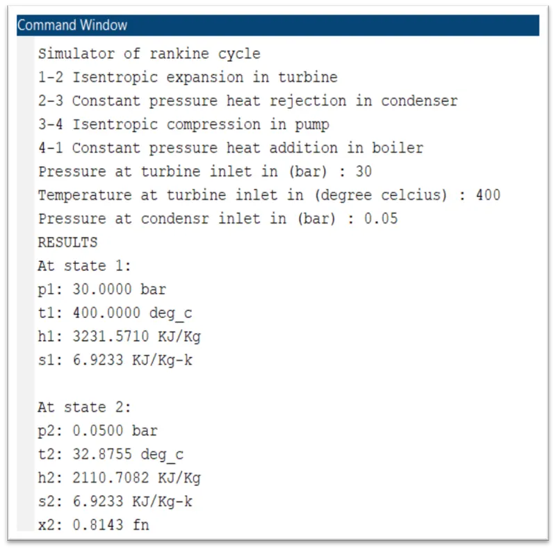
When Given values are as follows,

Inlet pressure in turbine = 30 bar

Inlet temp in turbine = 400 degree Celsius

Pressure in condenser = 0.05 bar

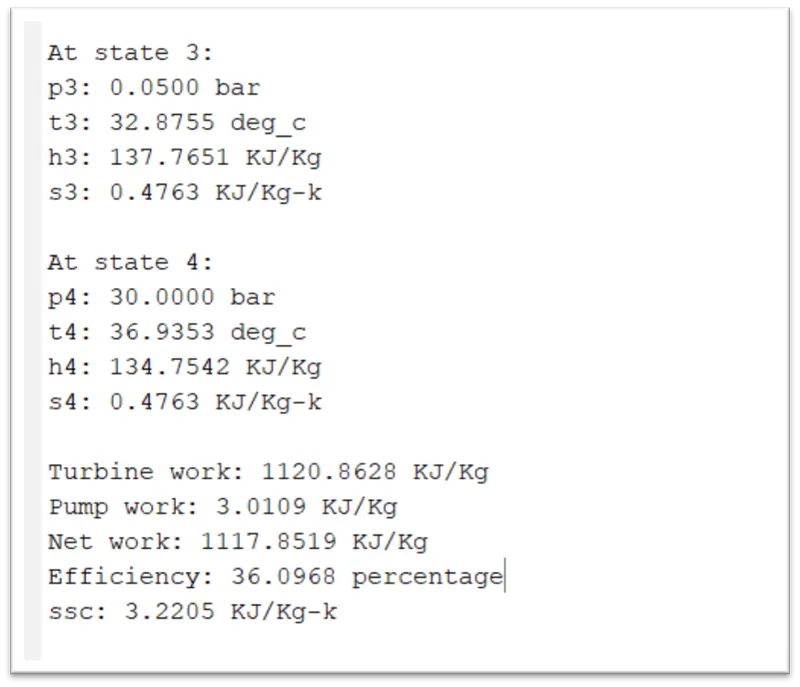
6.1 COMMAND WINDOW: -

6.2 PLOT: -

In above graph we see that from point 1 cycle started with turbine, here dry saturated steam from boiler was used to run turbine. heat is rejected in this process so temperature decreased from t1 to t2. Then in condenser the steam is converted in saturated liquid (water) that is t2 to t3 at constant pressure as the line is in under the saturated curve. Water is force by pump to boiler. here pressure is increased p3 to p4. In boiler water is converted into dry saturated steam that is t4 to t1 at constant pressure and then rotated the turbine. As temperature decrease entropy also decreased and when increased entropy also increased so the entropy is depended on temperature. The turbine work here is more than pump work always in cycle. The pump work is very small in this cycle.

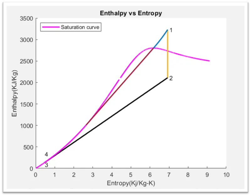
In above graph we can saw when pressure increased enthalpy also increased and when decreased the enthalpy also decreased, also Same for the entropy when temperature increased entropy also increased and when decreased the entropy also decreased So, we can say that enthalpy and entropy is totally depend on temperature and pressure. In turbine (1-2) pressure decreased so enthalpy also decreased at constant entropy. In condenser (2-3) temperature and pressure decreased so entropy and enthalpy also decreased. In pump (3-4) very small change in temperature and pressure increased.so the entropy and enthalpy change are also very small. But in boiler (4-1) temperature increased so the entropy also increased and practically when temperature is increased pressure also increased in cycle so entropy and enthalpy also increased simultaneously.

7. ERROR: -

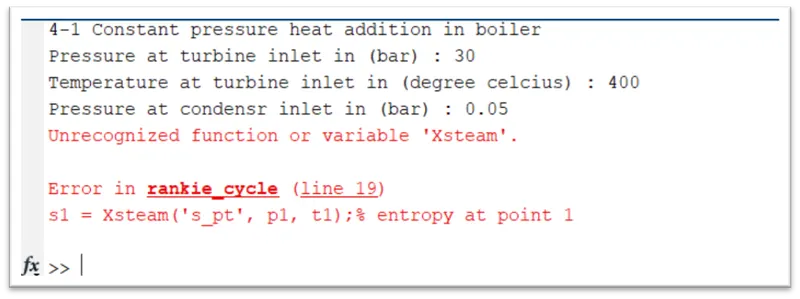
We know that the programming is case sensitive. This error occurred due to spelling mistake because our xsteam function is written wrong the function name. to overcome this error, we can write function name as XSteam.

8. CONCLUSION: -

We can conclude that MATLAB program for Rankine cycle computed and this code helps to design the power plant operating condition by which the plant efficiency can be increased and specific steam consumption can be decreased.

9. REFERENCE: -

• Web link

https://drive.google.com/file/d/1RK_fvrOj38CIaQvmLT1S3daqHnxKCGU-/view

http://www.powerfromthesun.net/Book/chapter12/chapter12.html

https://www.youtube.com/watch?v=MQ13EepiG9Q

• Books

Engineering Thermodynamics Fifth Edition - P K Nag

Engineering Thermodynamics – R K Rajput