MATLAB PROGRAM FOR CURVE FITTING

1. AIM: -

Write code to fit a linear and cubic polynomial for the Cp data

2. OBJECTIVE: -

• Plot the linear and cubic fit curves along with the raw data points.
• Write a code to show split wise method.
• Explain the parameters used to measure the fitness characteristics for both the curves.

3. GOVERNING EQUATION: -

• Linear polynomial (1^st degree of polynomial)

A linear polynomial is defined as any polynomial expressed in the form of an equation of `p(x) = ax + b`, where a and b are real numbers and a ≠ 0. In a linear polynomial, the degree of the variable is equal to 1 i.e., the highest exponent of the variable is one.

• Quadratic polynomial (2^nd degree of polynomial)

A Quadratic polynomial is defined as any polynomial expressed in the form of an equation of `p(x)= ax^2 + bx+c`, where a, b and c are real numbers and a, b ≠ 0. In a Quadratic polynomial, the degree of the variable is equal to 2 i.e., the highest exponent of the variable is one.

• Cubic polynomial (3^rd degree of polynomial)

A Cubic polynomial is defined as any polynomial expressed in the form of an equation of `p(x)= ax^3 + bx^2+cx+d`, where a, b, c, and d are real numbers and a, b, c ≠ 0. In a Cubic polynomial, the degree of the variable is equal to 3 i.e., the highest exponent of the variable is one.

4. DESCRIPTION: -

4.1 Curve fit

Curve fitting is the process of creating a curve, or mathematical function, that has the best fit to the data points, possibly subject to constraints. Curve fitting can involve either interpolation, where an exact best fit the trend of a given set of data, or smoothing spline, in which a "smooth" function is constructed that approximately fits the data. A related topic is regression analysis, which focuses more on questions of statistical inference such as how much uncertainty is present in a curve that is fit to data observed with random errors. Fitted curves can be used as an aid for data visualization, to infer values of a function where no data are available, and to summarize the relationships among two or more variables. Extrapolation refers to the use of a fitted curve beyond the range of the observed data, and is subject to a degree of uncertainty since it may reflect the method used to construct the curve as much as it reflects the observed data.

Curve fitting is one of the most powerful and most widely used analysis tools in Origin. Curve fitting examines the relationship between one or more predictors (independent variables) and a response variable (dependent variable), with the goal of defining a "best fit" model of the relationship.

4.2 Fitness Characteristics

• Sum of Squares Error (SSE)

`∑_(i=1)^n(Y(i)-f(x(i)))^2`

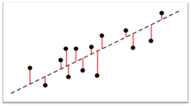
Sum of Squares Due to Error. This statistic measures the total deviation of the response values from the fit to the response values. It is also called the summed square of residuals and is usually labelled as SSE

• R-Square

R-square is the square of the correlation between the response values and the predicted response values. It is also called the square of the multiple correlation coefficient and the coefficient of multiple determination.

The R-squared, also called the coefficient of determination, is used to explain the degree to which input variables (predictor variables) explain the variation of output variables (predicted variables). It ranges from 0 to 1. For example, if the R-squared is 0.9, it indicates that 90% of the variation in the output variables are explained by the input variables. Generally speaking, a higher R-squared indicates a better fit for the model.

`R^2=(SSR)/(SST)`

Were,

SSR: - Sum of Square of Regression, which is basically the square of the difference between the value of the fitting function at a given point and the arithmetic mean of the data set.

`SSR= ∑_(i=1)^n(f(x(i))-Mean)^2`

SST: - Sum of Squares Total, the rationale is the following: the total variability of the data set is equal to the variability explained by the regression line plus the unexplained variability, known as error.

`SST= SSR+SSE`

SSE: - Sum of Squares Error, the error is the difference between the observed value and the predicted value

`∑_(i=1)^n(Y(i)-f(x(i)))^2`

• Adjusted R Square

Adjusted R-squared is a modified version of R-squared that has been adjusted for the number of predictors in the model. The adjusted R-squared increases when the new term improves the model more than would be expected by chance. It decreases when a predictor improves the model by less than expected. Typically, the adjusted R-squared is positive, not negative. It is always lower than the R-square.

R2 shows how well terms (data points) fit a curve or line. Adjusted R2 also indicates how well terms fit a curve or line, but adjusts for the number of terms in a model. If you add more and more useless variables to a model, adjusted r-squared will decrease. If you add more useful variables, adjusted r-squared will increase. Adjusted R2 will always be less than or equal to R2

R2 assumes that every single variable explains the variation in the dependent variable. The adjusted R2 tells you the percentage of variation explained by only the independent variables that actually affect the dependent variable.

`R^2 adj=1-[(1-R^2 )(n-1)/(n-k-1)]`

Where,

N = No. of points in your data sample

K = No. of independent variables

• Root Mean Squared Error (RMSE)

Also called as Root Mean Square Deviation (RMSD)

`RMSE= √(∑_(i=1)^n(Y(i)-f(x(i)))^2/n)`

`RMSE= √((SSE)/n)`

Were,

n = total no. of datapoint available

Root Mean Square Error (RMSE) is the standard deviation of the residuals (prediction errors). Residuals are a measure of how far from the regression line data points are; RMSE is a measure of how spread out these residuals are. In other words, it tells you how concentrated the data is around the line of best fit. Root mean square error is commonly used in climatology, forecasting, and regression analysis to verify experimental results.

5. QUESTION

5.1 How to make a curve fit perfectly?

Ans: - to make curve fit perfect we can use splitwise method with scaling and centering for curve fit. With help of mean and standard deviation we can get perfect fit. In R-Square method, when R-Square value is 1 then the curve is considered to be perfect. Here the given data curve and predicted data curve is perfectly match without any error. If any error occurs, we can use centering and scaling method.

5.2 How to get the best fit?

Ans: - to get the best fit we can use split wise method for curve fit also we can use following method

• Sum Squares Error (SSE)
• R Square
• Adjusted R Square
• Root Mean Squared Error (RMSE)

If he R square value is greater than 0.95 then we can consider curve to be best.

5.3 What could be done to improve the cubic fit?

To improve the cubic fit, we can use split wise method for curve fit. We can normalise the data with the help of scaling and centring method to overcome the error for increasing polynomial. We can also use curve fitting toolbox for curve fitting.

6. PROGRAM

6.1 LINEAR POLYNOMIAL

clear All
close all
clc

% Preparing a data
cp_data = load("data");
temperature = cp_data(:,1);
cp = cp_data(:,2);

% figure (1)
% 1st order polynomial
% cp = a*T + c
co_effs1 = polyfit(temperature,cp,1);
predicted_cp1 = polyval(co_effs1,temperature);

%compare my curve fit and given data
plot(temperature,cp,'linewidth',3,'color','black');
hold on
plot(temperature,predicted_cp1,"linewidth",3,'color','r')
xlabel('Temperature[k]')
ylabel('Specific heat[kj/kmol-k]')
legend('original data', 'curve fit linear')
title('Linear polynomial for cp data')

% checking eror for curve fit linear
disp('for the linear curve fit we have found: ')
curvefit_error_function(cp,predicted_cp1)

% Percentage of Error
error = (cp-predicted_cp1).*100./cp;
fprintf('max error percentage')
disp(max(error));

6.2 Function command for R square value

function curvefit_error_function(cp,predicted_cp)
meancp = mean(cp);
ssr = 0;
sse = 0;
for i = 1:length(cp)
    sse = sse+(cp(i)-predicted_cp(i))^2;
end
for i = 1:length(cp)
    ssr = ssr+(meancp-predicted_cp(i))^2;
end
sst = sse+ssr;
rssquare = ssr/sst

if (rssquare>0.95)
    disp('The curve fit is good');
else ;disp('The curve fit is not good')
end

6.3 EXPLANATION

• Firstly, we used clearvars, close all, clc, to clear workspace, graphs and command window.
• Loaded a cp data in program with ‘load’ command.
• Gave variable to temperature and specific heat.
• Took coefficient and predicted cp for linear polynomial with the help of polyfit and polyval command.
• Compared curve fit with given data with plotting graph for temperature vs cp and temperature vs predicted cp.
• Used function command to check error for curve fit with the help of R-square formula. also used for loop and if else command.
• Checked max error percentage with help of Fprintf and disp command to display result in command window.

6.4 Output for linear polynomial

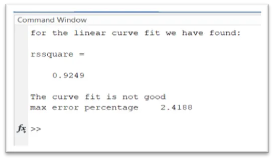
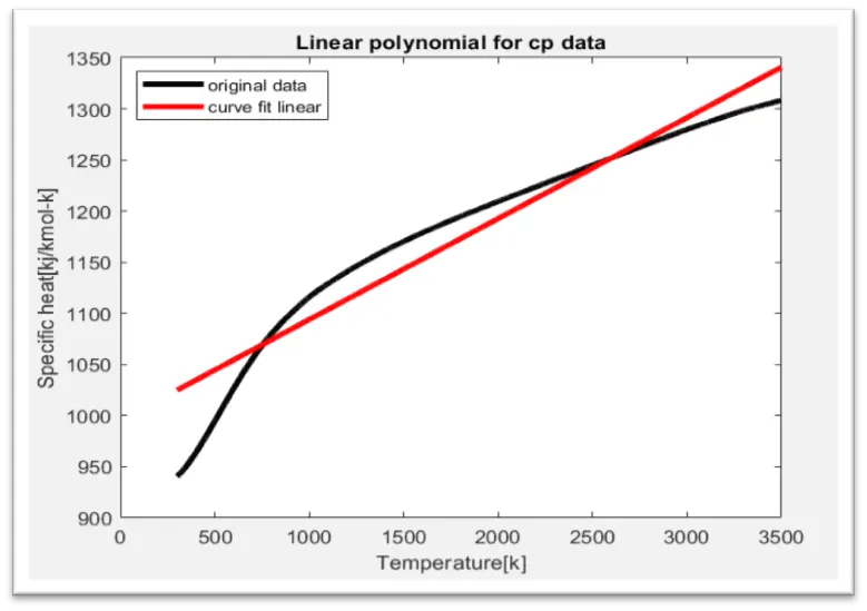
Here we get results for our program. For linear curve fit we have fond r square = 0.9249, so the curve fit is not good. because if r square is greater than 0.95 then only the fit is good. Max error percentage is 2.4188 was also not good.

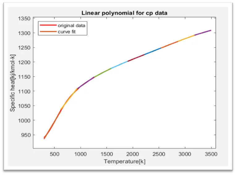
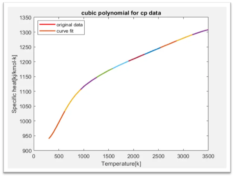
6.5 Split wise method for the cp data

To overcome this problem, we have to split our data in some parts that’s call split wise method. Where we split curve into multiple no. of polynomials for a different set of temperature value. The main factor of splitting is the no. of divisions. By ensuring more split of the data a higher accuracy of output curve can be achieved.

clearvars
close all
clc
%curve fitting split wise polynomial
cp_data = load("data");
temperature = cp_data(:,1);
cp = cp_data(:,2);
plot(temperature,cp,'linewidth',2,'Color','r')

% split the cp value in 10 parts
a = 1;
b = 3200/10;
for i = 1:10
    new_temperature = cp_data(a:b,1);
    new_cp = cp_data(a:b,2);
    
    hold on
    [co_effs,~,mu] = polyfit(new_temperature,new_cp,1);
    predicted_cp = polyval(co_effs,new_temperature,[],mu);
    a = 1+b;
    b = b+320;
    plot(new_temperature,predicted_cp,'linewidth',2);
    xlabel('Temperature[k]')
    ylabel('Specific heat[kj/kmol-k]')
    legend('original data', 'curve fit')
    title('linear polynomial for cp data')
    
end
% checking eror for curve fit linear
disp('for the linear polynomial curve fit we have found: ')
curvefit_error_function(new_cp,predicted_cp)

% Percentage of Error
error = (new_cp-predicted_cp).*100./new_cp;
fprintf('max error percentage')
disp(max(error));

6.6 Output of Splitting

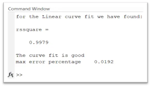
Here we get results for our program. For linear curve fit with split wise method we have fond r square = 0.9979, so the curve fit is good. because if r square is greater than 0.95 then only the fit is good. Max error percentage is 0.0192 was also good. We obtain a best fit for linear polynomial

7. CUBIC POLYNOMIAL

clear All
close all
clc

% Preparing a data
cp_data = load("data");
temperature = cp_data(:,1);
cp = cp_data(:,2);

% figure (1)
% 1st order polynomial
% cp = a*T + c
co_effs1 = polyfit(temperature,cp,1);
predicted_cp1 = polyval(co_effs1,temperature);

% figure (3)
% 3st order polynomial
% cp = a*T^3 + b*T^2 + c*T + d
co_effs3 = polyfit(temperature,cp,3);
predicted_cp3 = polyval(co_effs3,temperature);

%compare my curve fit and given data
plot(temperature,cp,'linewidth',3,'color','black');
hold on
plot(temperature,predicted_cp3,"linewidth",3,'color','r')
xlabel('Temperature[k]')
ylabel('Specific heat[kj/kmol-k]')
legend('original data', 'curve fit cubic')
title('Cubic polynomial for cp data')

% checking eror for curve fit cubic
disp('for the cubic curve fit we have found: ')
curvefit_error_function(cp,predicted_cp3)

% Percentage of Error
error = (cp-predicted_cp3).*100./cp;
fprintf('max error percentage')
disp(max(error));

7.1 EXPLANATION

• Here we used same program and command which we used for linear polynomial. Only the change is coefficient for cubic polynomial. Change is as above program,

7.2 Output for Cubic Polynomial

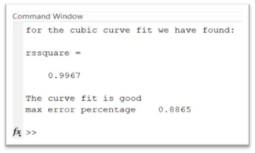
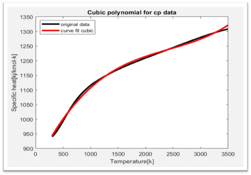
Here we get results for our program. For cubic curve fit we have fond r square = 0.9967, so the curve fit is best. because if r square is greater than 0.95 then only the fit is best. Max error percentage is 0.8865 was also good. When error is decreasing, we get best fit for curve.

Usually, if the R square is greater than 0.95 then the curve fit is considered to be best. And if the R square value is 1 then the curve fir id considered to e perfect.

7.3 Splitting the cp data

For perfect curve fit we are used split wise method as follow,

clearvars
close all
clc
%curve fitting split wise polynomial
cp_data = load("data");
temperature = cp_data(:,1);
cp = cp_data(:,2);
plot(temperature,cp,'linewidth',2,'Color','r')

% split the cp value in 10 parts
a = 1;
b = 3200/10;
for i = 1:10
    new_temperature = cp_data(a:b,1);
    new_cp = cp_data(a:b,2);
    
    hold on
    co_effs = polyfit(new_temperature,new_cp,3);
    predicted_cp = polyval(co_effs,new_temperature);
    a = 1+b;
    b = b+320;
    plot(new_temperature,predicted_cp,'linewidth',2);
    xlabel('Temperature[k]')
    ylabel('Specific heat[kj/kmol-k]')
    legend('original data', 'curve fit')
    title('Cubic polynomial for cp data')
    
end
% checking eror for curve fit Cubic
disp('for the Cubic polynomial curve fit we have found: ')
curvefit_error_function(new_cp,predicted_cp)

% Percentage of Error
error = (new_cp-predicted_cp).*100./new_cp;
fprintf('max error percentage')
disp(max(error));

7.4 Output

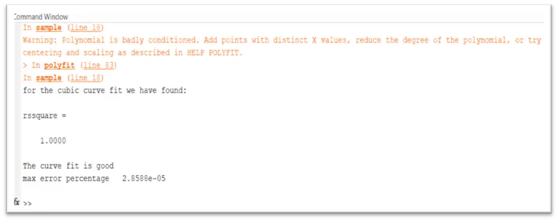
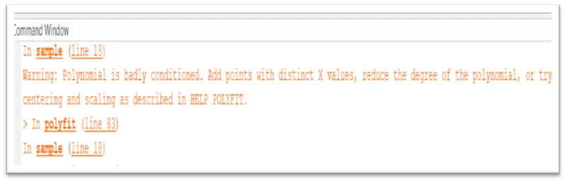
Here we get results for our program. For cubic curve fit with split wise method we have fond r square = 1, so the curve fit is perfect. because if r square is equal to 1 then only the fit is perfect. Max error percentage is 2.8588e-05 was also best. We obtain a perfect fit for cubic polynomial but we get some error here as follow,

8. Error

9. Error Correction

Scaling and Centering

In this process we normalise the data with the help of mean and standard deviation.

Use polyfit with outputs to fit a 3th-degree polynomial using centering and scaling, which improves the numerical properties of the problem. polyfit centers the data in cp at 0 and scales it to have a standard deviation of 1,

[co_effs,~,mu] = polyfit(new_temperature,new_cp,3);

predicted_cp = polyval(co_effs,new_temperature,[],mu);

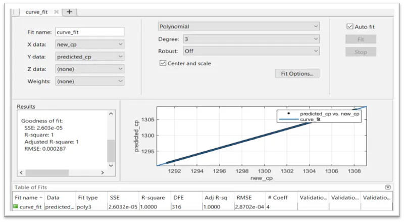
10. Curve fit Toolbox

This is another alternative to validate the fitness characteristics of curve fitting.

Curve Fitting Toolbox provides an app and functions for fitting curves and surfaces to data. The toolbox lets you perform exploratory data analysis, pre-process and post-process data, compare candidate models, and remove outliers. You can conduct regression analysis using the library of linear and nonlinear models provided or specify your own custom equations. The library provides optimized solver parameters and starting conditions to improve the quality of your fits. The toolbox also supports nonparametric modelling techniques, such as splines, interpolation, and smoothing.

After creating a fit, you can apply a variety of post-processing methods for plotting, interpolation, and extrapolation; estimating confidence intervals; and calculating integrals and derivatives.

11. CONCLUSION

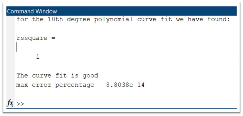
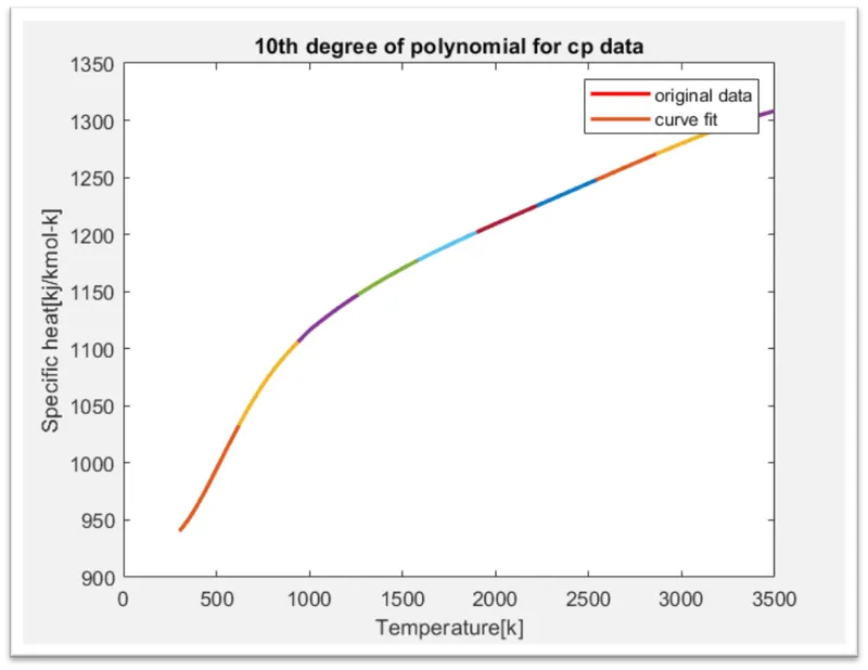
Here we conclude that, we can obtain perfect curve fit for linear and cubic polynomial with the help of above program. simple change in polynomial we can use this program for multiple degree of polynomial as follow

clearvars
close all
clc
%curve fitting split wise polynomial
cp_data = load("data");
temperature = cp_data(:,1);
cp = cp_data(:,2);
plot(temperature,cp,'linewidth',2,'Color','r')

% split the cp value in 10 parts
a = 1;
b = 3200/10;
for i = 1:10
    new_temperature = cp_data(a:b,1);
    new_cp = cp_data(a:b,2);
    
    hold on
    [co_effs,~,mu] = polyfit(new_temperature,new_cp,10);
    predicted_cp = polyval(co_effs,new_temperature,[],mu);
    a = 1+b;
    b = b+320;
    plot(new_temperature,predicted_cp,'linewidth',2);
    xlabel('Temperature[k]')
    ylabel('Specific heat[kj/kmol-k]')
    legend('original data', 'curve fit')
    title('10th degree of polynomial for cp data')
    
end
% checking eror for curve fit cubic
disp('for the 10th degree polynomial curve fit we have found: ')
curvefit_error_function(new_cp,predicted_cp)

% Percentage of Error
error = (new_cp-predicted_cp).*100./new_cp;
fprintf('max error percentage')
disp(max(error));

11.1 OUTPUT

12. REFERENCES

https://skill-lync.com/student-projects/Curve-Fitting-and-criterion-to-choose-best-fit-41860

https://skill-lync.com/knowledgebase/curve-fit-toolbox-an-overview

https://skill-lync.com/knowledgebase/the-basic-concept-of-curve-fit

https://skill-lync.com/student-projects/linear-and-cubic-curve-fitting-for-the-cp-data-using-matlab