Final Project: Design of an Electric Vehicle

1. AIM: -

To design an Electric vehicle Using MATLAB & Simulink.

2. OBJECTIVE: -

Create a MATLAB model of an electric car that uses a battery and a DC motor. Choose suitable blocks from the Powertrain block set. Prepare a report about your model including the following:

1. System-level configurations
2. Model parameters
3. Results
4. Conclusion

3. INTRODUCTION: -

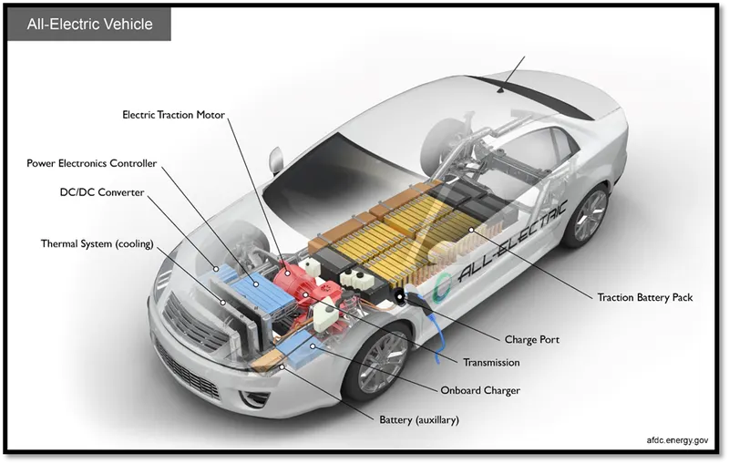
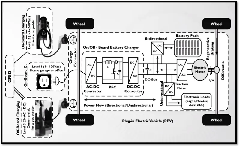
A pure electric vehicle (PEV), also known as an all-electric vehicle, operates solely on electricity as its name suggests. An on-board battery pack module (shown in the figure below) stores the electricity used to power the vehicle. The battery charge can be additionally extended while the vehicle is being operated through the regenerative braking system. Otherwise lost kinetic energy from braking is saved in a storage battery which can be used later to power the motor when in need. When the vehicle is not in use, the battery pack is recharged by plugging the vehicle into an external electric power source such as a charging station or a home outlet.

Since pure electric vehicles do not have a gasoline engine, they do not have tailpipe emissions (they do not possess a tailpipe). However, these vehicles do cause emissions that take place elsewhere, such as at the electric power plant and the manufacturing facility (most of them originating from the battery’s construction) with amounts varying greatly based on the source of electricity and energy used. All-electric vehicles are more energy efficient

compared to conventional gasoline vehicles, as they can convert about 59%-62% of the electrical energy provided by the grid to power the wheels, whereas a typical gasoline vehicle can only convert about 17%-21% of the energy stored in gasoline to useful power.

Their driving range on a full charge typically ranges between 60-100 miles, according to the most recent (2015) available models, with a few exceptions which can reach up to 200-300 miles, as in the Tesla Model S with a boasting rating of 270 miles on a full battery charge. According to the charging technology used, fully recharging the vehicle’s battery pack typically takes between 4-8 hours. There is the option of what is known as a ‘superfast charge’, which can recharge the vehicle’s battery to 80% capacity in about 30 minutes.

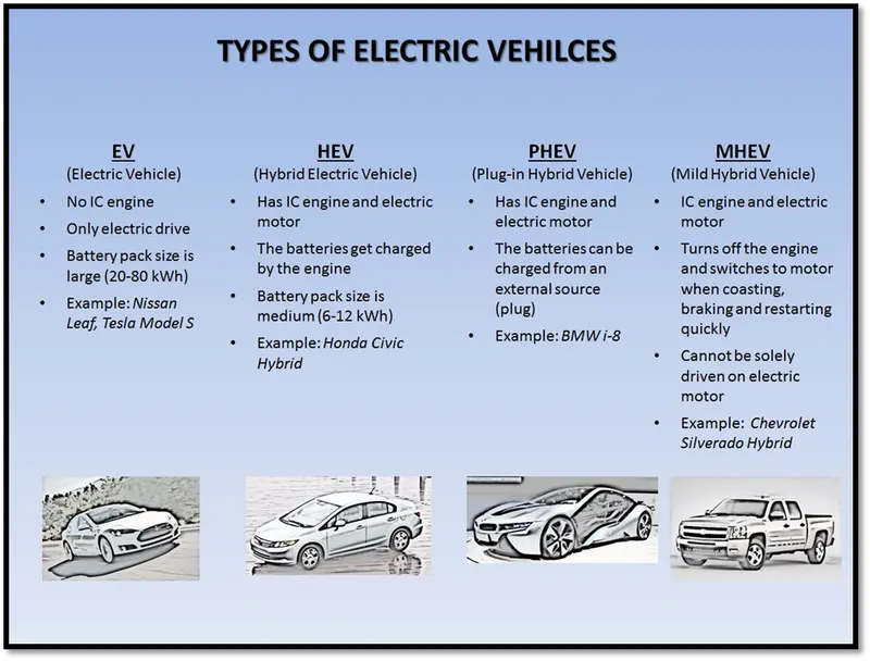
3.1 Types of Electric Vehicle: -

3.2 The architecture of Electric Vehicle: -

3.3 Block diagram for model: -

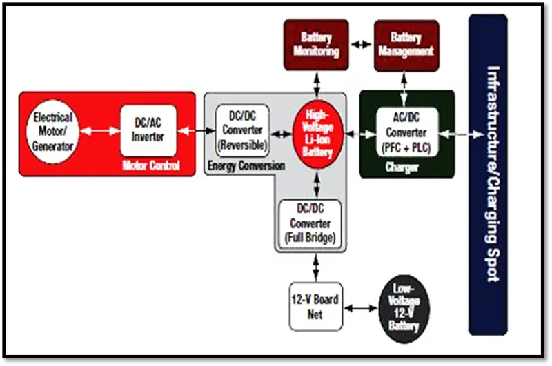
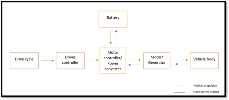
There are several components and a vast network of connecting wires in the electric vehicle. In the case of an electric vehicle, the conventional IC engine is replaced by a motor. The working fuel that is the battery pack is supplied to the motor. The block diagram below will show significant components of the Electric Vehicle system.

The key components of electric vehicles are the motor, vehicle body, controller, and battery pack. There are several types of motors used in Electric Vehicles. BLDC motors, Brushed DC motors, and AC Induction Motors are commonly used electric motors. The vehicle body includes a gearbox, differentials, and tires. Earlier, we used the battery just to start the engine. But now we are using the battery as a working power. Combinations of cells will create a module, and many modules will form a battery pack together. The motor needs a power supply from the battery to perform operations. Suppose we connect the battery pack directly to the motor. In that case, the motor will run at a rated speed, and speed control is not possible. We can control the speed of the motor with the aid of the controller. The controller will operate by taking input from the driver.

3.4 The main component of EV: -

1. Battery
2. Power converter
3. Motor controller
4. Motor / Generator
5. Vehicle body (tire /transmission)

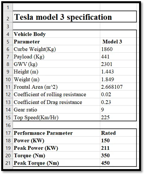
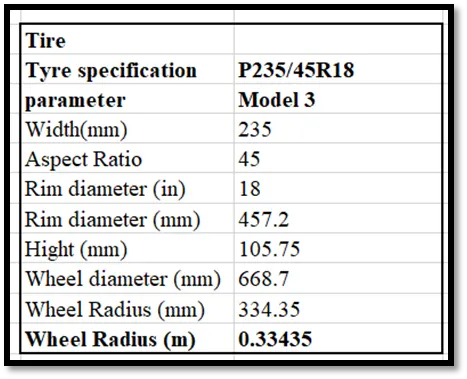
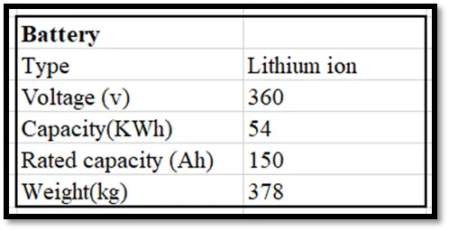
• Data used: - Tesla model 3
• Tesla Model 3 RWD (2021)

4. SIMULINK MODEL: -

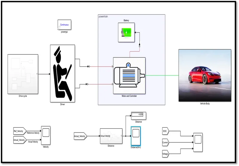
1. In this model have designed an EV (Tesla Model 3) which runs based on the FTP75 drive cycle. It goes to Vehicle reference of Longitudinal driver block.
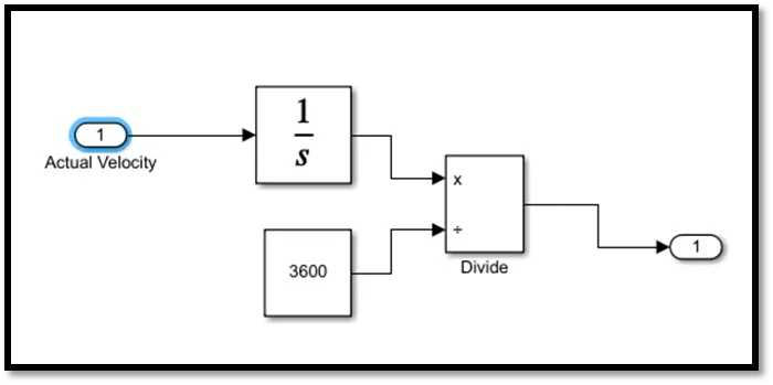
2. Speed is taken as feedback through a Simulink-PS converter from the Vehicle subsystem and given grade ability 0. For distance calculation, an integrator block and a constant are connected with the Divide block's multiply and divide terminal respectively.
3. Acceleration Command is given to the Control Voltage source through a Simulink-PS Converter. The negative of the Control voltage source is grounded.
4. Then Deacceleration command from the Longitudinal driver is sent to another Control voltage source2 through a Simulink-PS converter. The negative of Control voltage source2 is grounded.
5. Positive signal of the Control voltage source land Control voltage source2 sends to Controlled PWM voltage as a positive reference and H-Bridge as braking command respectively.
6. Negative reference of Control PWM voltage, Reverse of H-Bridge, and both Reference output of Control PWM voltage and H-Bridge is grounded.
7. A solver configuration is connected to the ground. Reference output of Control PWM voltage and H-Bridge is connected. Two output ports of H-Bridge are connected to a DC motor's two terminals. Also, the positive output of the H-bridge is connected to a controlled current source through a current sensor.
8. From the current sensor, the current is sent to the Battery block through a PS-Simulink converter. Positive and negative of the battery and controlled current source are connected inversely to each other.
9. Then negative is grounded port of the DC motor is attached with a mechanical rotational reference and R port torque is sent to the Gearbox (G) of the vehicle body subsystem.
10. Vehicle body subsystem is created with a standard block in MATLAB. 4 tires blocks and vehicle body block connected with proper terminal.

5. SYSTEM-LEVEL CONFIGURATION: -

5.1 Vehicle body: -

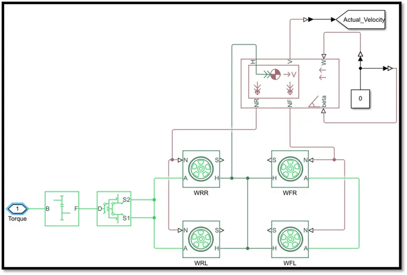
1. The vehicle body subsystem was created with the help of tire, vehicle body, differential, and simple gear blocks.
2. Connection A is the mechanical rotational conserving port for the wheel axle.
3. Connection H is the mechanical translational conserving port for the wheel hub through which the thrust developed by the tire is applied to the vehicle.
4. Connection N is a physical signal input port that applies the normal force acting on the tire. The force is considered positive if it acts downwards.
5. Connection S is a physical signal output port that reports the tire slip.
6. 4 tire blocks are added to the subsystem. The H connection of all tires is connected with the vehicle body's H port.
7. Rear-wheel N connection is connected to NR and Front wheel N connection to NF.
8. Constant blocks are connected to the Wind velocity(W) and Gradeability (Beta) ports through the Simulink-PS converter.
9. The rear wheel A connection is connected. The front wheel is also connected the same as the rear wheel.
10. The connection V is vehicle speed which is connected to the outside display with the help of a PS-Simulink converter to change the physical signal to a digital quantity. We took the unit for the converter is km/hr.
11. The torque from the motor is given to simple gear and then differential. Most of the EVs are now direct giving power to the wheel so the differential used is negligible. For that reason, take differential ratio 1 or we can also develop a model without differential block.

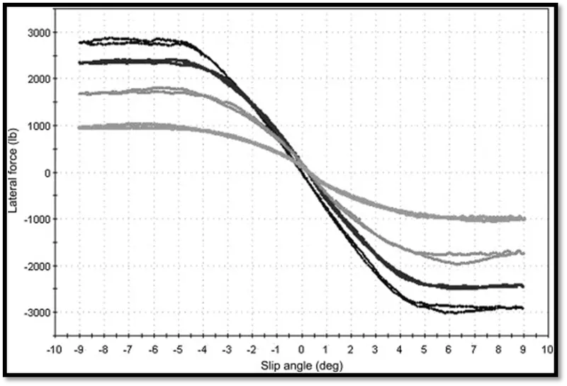
• Tire magic formula: -

The generic Magic Formula has been developed using mathematical functions that relate to:

1. The lateral force Fy as a function of slip angle α.
2. The aligning moment Mz as a function of slip angle α.
3. The longitudinal force Fx as a function of longitudinal slip κ.

When these curves are obtained from steady-state tire testing and plotted, the general shape of the curves is similar to that indicated below figure. It is important to note that the data used to generate the tire model is obtained from steady-state testing. The lateral force Fy and the aligning moment Mz are measured during pure cornering, i.e. cornering without braking, and the longitudinal braking force during pure braking, i.e. braking without cornering.

5.2 Motor with controller: -

The PMSM has low torque repulsion so PMSM got higher and smooth torque with higher efficiency and low noise compared to BLDCM. PMSM has a higher power density, which will help in reducing the size of the motor. That’s why PMSM is better than BLDC motor in terms of performance and is good to use in electric vehicles.

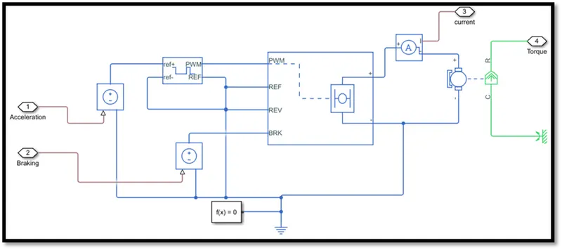
1. The motor and controller subsystem was created with the help of a dc motor, H bridge, controlled PWM voltage, controlled voltage source, and current sensor blocks.
2. Acceleration and deacceleration both inputs from longitudinal driver block go to controlled voltage source 1 and 2 to the input of controlled PWM voltage and braking of H bridge block.
3. H bridge block is connected with DC motor and current sensor, the further current sensor is connected with battery source with the help of controlled current source and PS – Simulink converter.
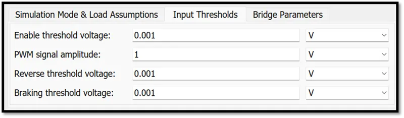
4. If the REV port voltage is greater than the Reverse threshold voltage, then the output voltage polarity is reversed.
5. If the BRK port voltage is greater than the Braking threshold voltage, then the output terminals are short-circuited via one bridge arm in series with the parallel combination of a second bridge arm and a freewheeling diode.
6. Voltages at ports PWM, REV, and BRK are defined relative to the REF port.
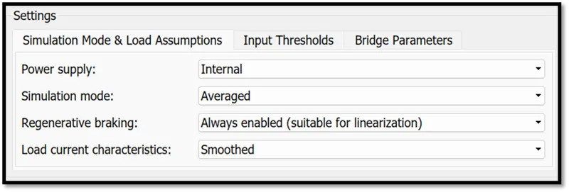
7. The Simulation mode parameter value must be the same for the Controlled PWM Voltage and H-Bridge blocks.
8. The PWM and H-bridge blocks are used to control the motor. we can give power supply to H-bridge internally or externally
9. The controlled voltage source is used to provide the same voltage throughout the circuit.

5.3 Battery: -

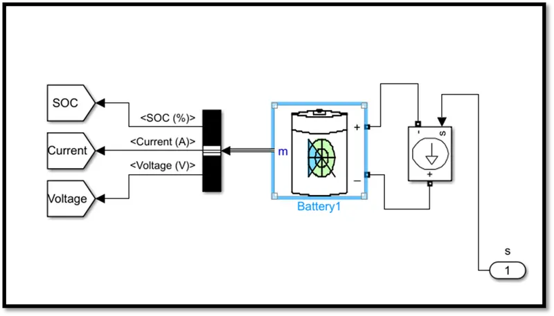
1. The battery subsystem was created with the help of batter, controlled current source, and bus selector block.
2. I used a battery that can directly give soc, current, and voltage data to the user.
3. Bus selector is used to select which data we need from the battery to display to the user.
4. Go to tag is used with global tag visibility to send outside the subsystem.
5. Current controlled source here also works as a control voltage source.

5.4 Driver: -

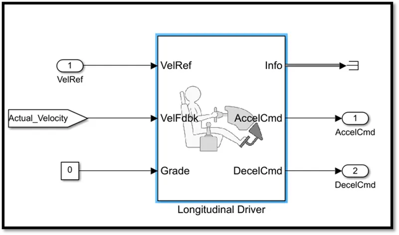
1. I used here a longitudinal driver block that is standard in Simulink work as a driver for the vehicle to respond to all systems.
2. Also used from, terminator, inport an outport block to connect the subsystem.
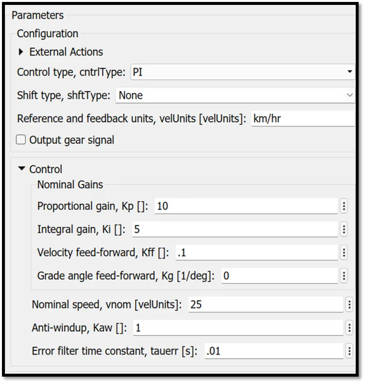
3. A parametric longitudinal speed tracking controller for generating normalized acceleration and braking commands based on reference and feedback velocities.
4. Use external actions to input signals that can disable, hold, or override the closed-loop commands determined by the block. The block uses this priority for the input commands: disable, hold, override.

5.5 Drive cycle: -

A driving cycle is a series of data points representing the speed of a vehicle versus time. Driving cycles are produced by different countries and organizations to assess the performance of vehicles in various ways, for instance, fuel consumption, electric vehicle autonomy, and polluting emissions Fuel consumption and emission tests are performed on chassis dynamometers. Tailpipe emissions are collected and measured to indicate the performance of the vehicle. Another use for driving cycles is in vehicle simulations. More specifically, they are used in propulsion system simulations to predict the performance of internal combustion engines, transmissions, electric drive systems, batteries, fuel cell systems, and similar components.

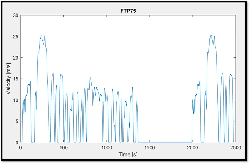
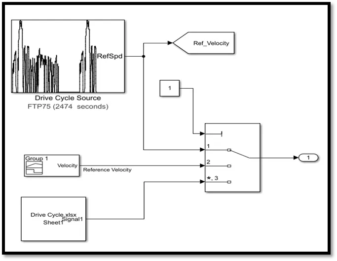
1. Here we used the multiport switch to change the input to reference velocity of the driver subsystem.
2. Three different inputs were used which are drive cycle source, signal builder, and from a spreadsheet.
3. With the help of the speed sheet and signal builder, we can build our own drive cycle.
4. We connect the constant block to the switch to give input.
5. Here we have to be careful which drive cycle we are using has to be connected with reference velocity goto block so we can match the reference and actual velocity.
6. Also, we have to change the simulation time accordingly.

5.6 Distance calculation: -

 

6. MODEL PARAMETER: -

 

6.1 Tire: -

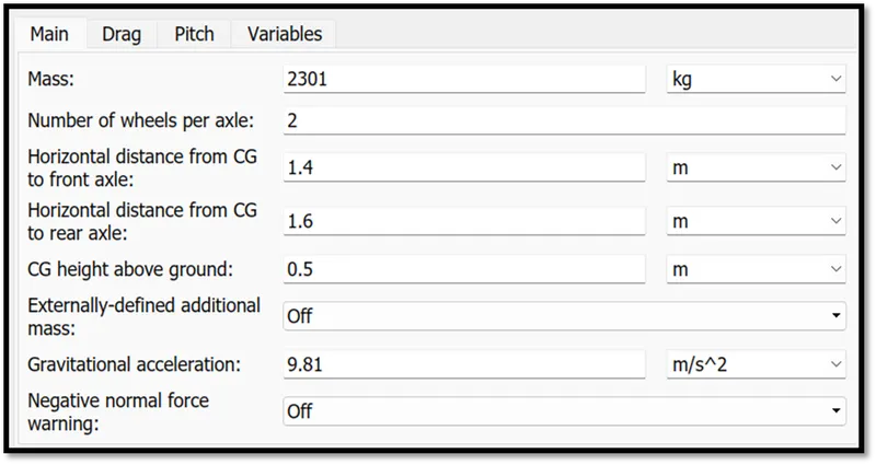
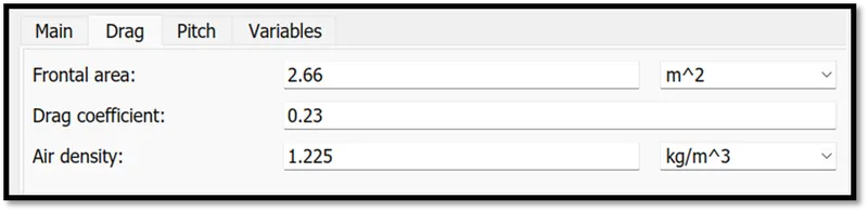
6.2 Vehicle body: -

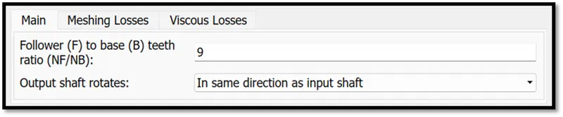
6.3 Simple gear: -

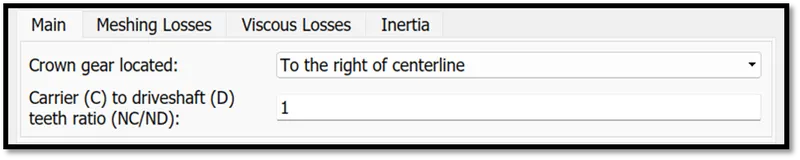
6.4 Differential: -

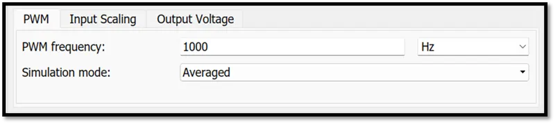
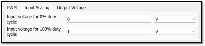
6.5 Controlled PWM voltage: -

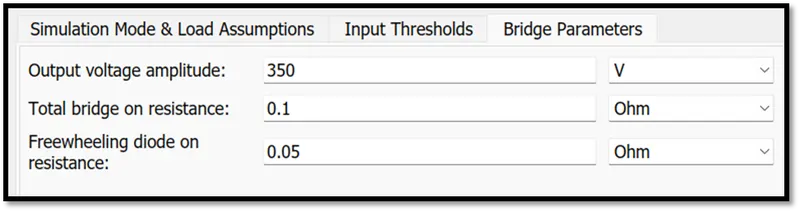
6.6 H-bridge: -

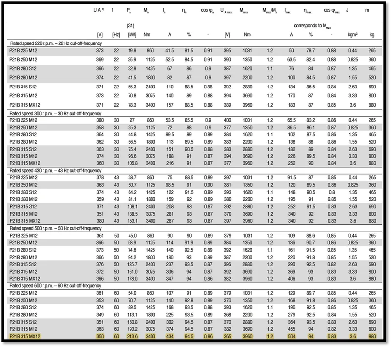
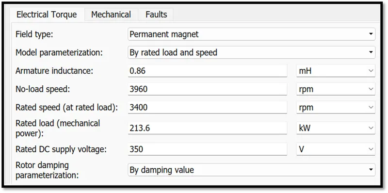
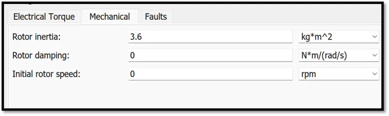
6.7 DC Motor: -

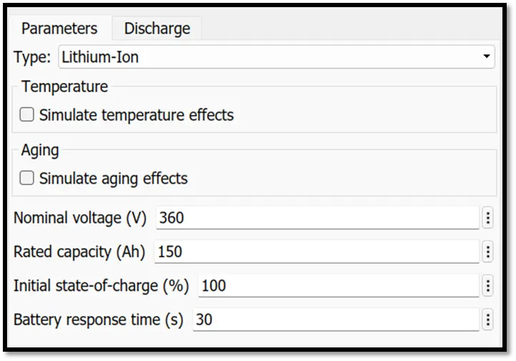
6.8 Battery: -

6.9 Longitudinal driver: -

7. Results: -

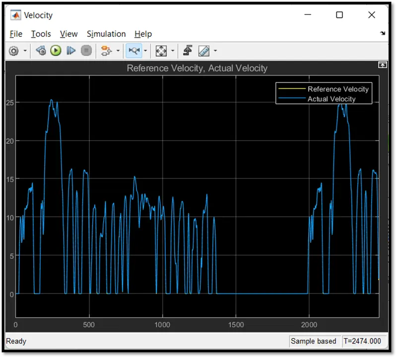
Here we can see that the actual velocity is closely following the reference velocity with very minor differences. The top speed of the vehicle is 25km/hr. If we increase the no-load speed the graph will follow the path exactly.

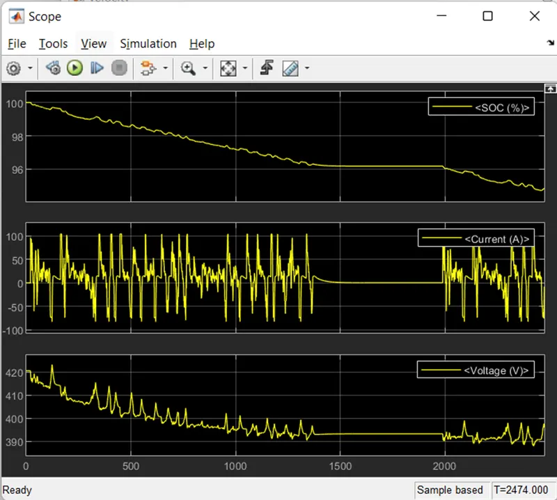
1. The soc of battery was decreased from 100-96 % but when current is negative the regenerative braking was happed so that battery is charging and soc will be increased.
2. If we see we can see soc following the current path. Also, if the voltage increases current will decrease which means when the battery is regenerative braking happens and the voltage goes increase.
3. At 1400 sec current was o till the2000 sec because velocity for this time is also zero.

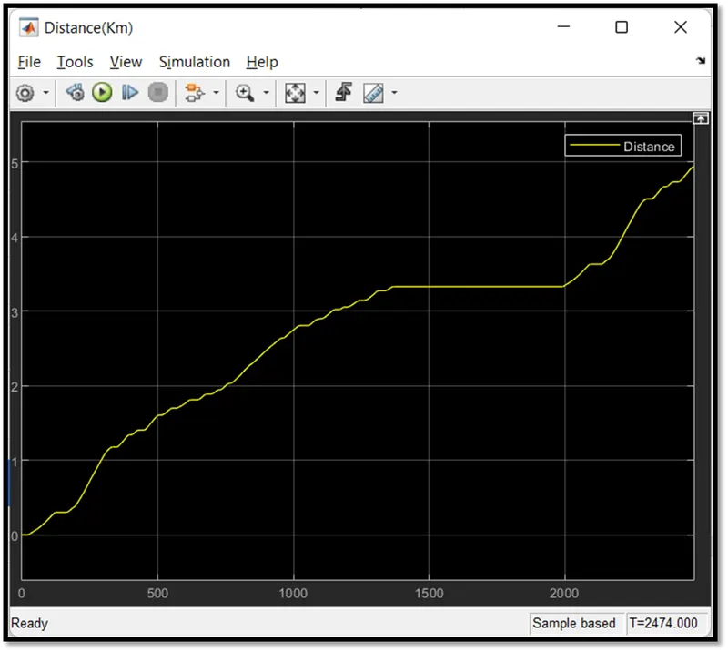
The vehicle covers a distance of 4.939 km in 2474 sec. if we gave constant speed at drive cycle input as 25km/hr without braking then we get almost a similar distance to 25 km.

8. CONCLUSION: -

The simulation model was created with a better result for electric vehicle design, we can also use different parameters to design the vehicle with better performance characteristics. This parameter can be changed. We can change the motor type, motor rating, controller rating, battery type and rating, drive cycle, etc. Based on those parameters the simulation result of SOC estimation, Current, Speed will change accordingly. We can use different batteries from the extra source directory and add other functions like a temperature sensor. As this is a pure EV, we can also make a hybrid EV and add other functions for simultaneously changing the operations of IC Engine and Motor.

We have examined the SOC percentage and speed graph. The SOC percentage graph indicates that the battery is discharged when there is an acceleration command. The battery is charged when there is a deceleration command. The Speed graph shows that the actual speed tries to meet the reference speed by considering feedback. The model shows that the electric vehicle has traveled approximately 5 km in 2474 seconds. If we measure the average speed, the vehicle will travel approximately 10 km/hr. This measured average speed is approximately equal to the reference average speed found on the graph.

9. Reference: -

• https://www.sciencedirect.com/topics/engineering/magic-formula#:~:text=The%20Magic%20Formula%20(Pacejka)%20tire,brake%2Fdrive)%20slip%20%CE%BA.
• Tesla Model 3 RWD (2021)
• https://en.wikipedia.org/wiki/Driving_cycle#Driving_Cycle_Design

10. EXCEL SHEET & EV MODEL ZIP file: -

https://drive.google.com/file/d/1GC_U31uxHiOD8DBl4eDsyhzPU0Xm6WXF/view?usp=sharing

11. Extra work: -

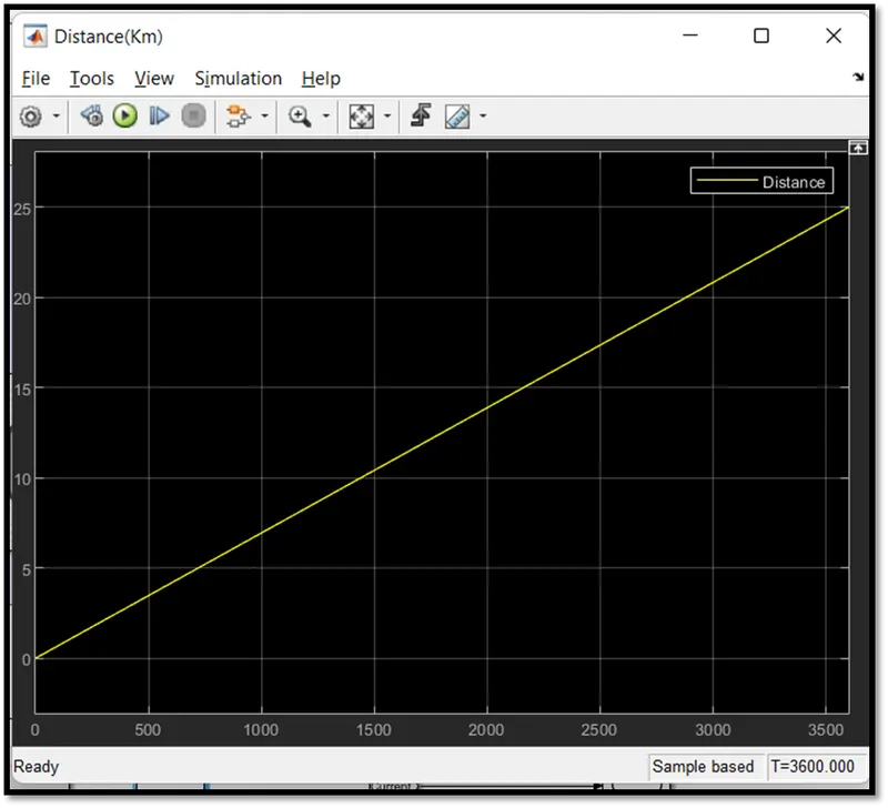
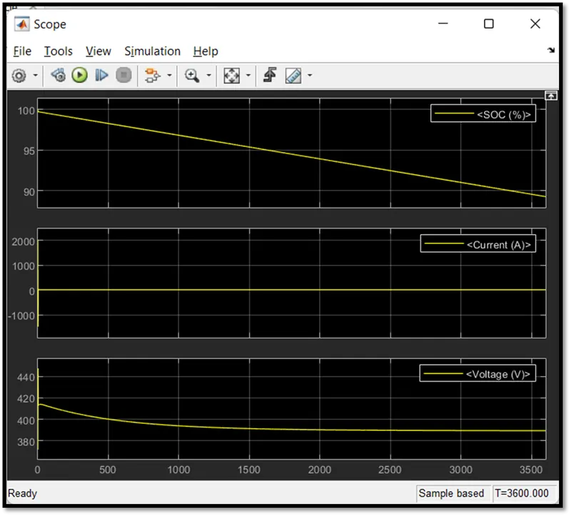
Constant speed drive cycle (25 km/hr)

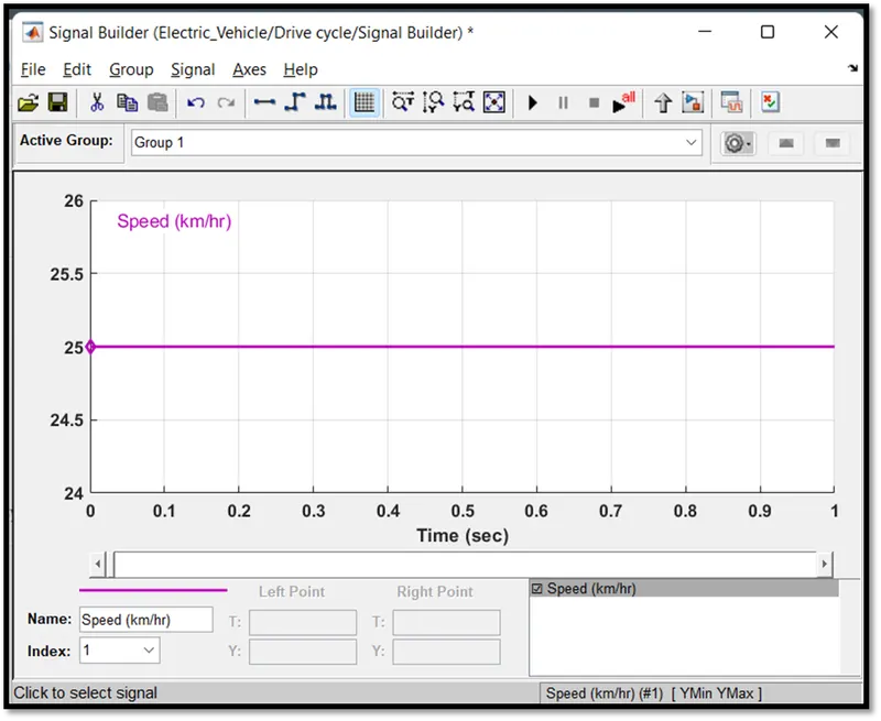
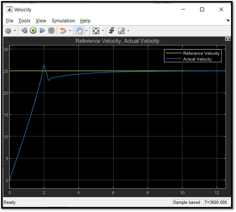
Here we can see to achieve the given speed its take 10 sec. after that It will be constant for 25 km/hr.