MATLAB PROGRAMING FOR GENETIC ALGORITHM OF STALAGMITE FUNCTION
1. AIM: -
Write a code in MATLAB to optimise the stalagmite function and find the global maxima of the function
2. OBJECTIVE: -
- Optimise the stalagmite function and find the global maxima of the function.
- Explain the concept of genetic algorithm and syntax for (ga) in MATLAB
- Make sure that your code gives the same output, even if it is made to run several times.
- Plot graphs for all 3 studies and for F maximum vs no. of iterations.
3. DESCRIPTION: -
3.1 Stalagmite Function
A stalagmite function generally refers to the function with which we are generating values over a stalagmite kind of surface for finding out the local and global maxima and minima of that particular given function.
3.2 Genetic Algorithm
The genetic algorithm is a method for solving both constrained and unconstrained optimization problems that is based on natural selection, the process that drives biological evolution. The genetic algorithm repeatedly modifies a population of individual solutions. At each step, the genetic algorithm selects individuals at random from the current population to be parents and uses them to produce the children for the next generation. Over successive generations, the population "evolves" toward an optimal solution. You can apply the genetic algorithm to solve a variety of optimization problems that are not well suited for standard optimization algorithms, including problems in which the objective function is discontinuous, nondifferentiable, stochastic, or highly nonlinear. The genetic algorithm can address problems of mixed integer programming, where some components are restricted to be integer-valued.
The genetic algorithm uses three main types of rules at each step to create the next generation from the current population:
- Selection rules select the individuals, called parents, that contribute to the population at the next generation.
- Crossover rules combine two parents to form children for the next generation.
- Mutation rules apply random changes to individual parents to form children.
3.3 Basic Terminology
Population: - It is a subset of all the possible (encoded) solutions to the given problem. The population for a GA is analogous to the population for human beings except that instead of human beings, we have Candidate Solutions representing human beings.
Chromosomes: - A chromosome is one such solution to the given problem.
Gene: - A gene is one element position of a chromosome.
Allele: - It is the value a gene takes for a particular chromosome.
Genotype: - Genotype is the population in the computation space. In the computation space, the solutions are represented in a way which can be easily understood and manipulated using a computing system.
Phenotype: - Phenotype is the population in the actual real-world solution space in which solutions are represented in a way they are represented in real world situations.
Decoding and Encoding: - For simple problems, the phenotype and genotype spaces are the same. However, in most of the cases, the phenotype and genotype spaces are different. Decoding is a process of transforming a solution from the genotype to the phenotype space, while encoding is a process of transforming from the phenotype to genotype space. Decoding should be fast as it is carried out repeatedly in a GA during the fitness value calculation.
Fitness Function: - A fitness function simply defined is a function which takes the solution as input and produces the suitability of the solution as the output. In some cases, the fitness function and the objective function may be the same, while in others it might be different based on the problem.
Genetic Operators: -These alter the genetic composition of the offspring. These include selection, crossover, mutation, etc
Parent Selection: - selections is the process of selecting parents which mate and recombine to create off-springs for the next generation. Parent selection is very crucial to the convergence rate of the GA as good parents drive individuals to a better and fitter solutions.
However, care should be taken to prevent one extremely fit solution from taking over the entire population in a few generations, as this leads to the solutions being close to one another in the solution space thereby leading to a loss of diversity. Maintaining good diversity in the population is extremely crucial for the success of a GA. This taking up of the entire population by one extremely fit solution is known as premature convergence and is an undesirable condition in a GA.
Crossover: - The crossover operator is analogous to reproduction and biological crossover. In this more than one parent is selected and one or more off-springs are produced using the genetic material of the parents. Crossover is usually applied in a GA with a high probability.
Mutation: - In simple terms, mutation may be defined as a small random tweak in the chromosome, to get a new solution. It is used to maintain and introduce diversity in the genetic population and is usually applied with a low probability – pm. If the probability is very high, the GA gets reduced to a random search. Mutation is the part of the GA which is related to the “exploration” of the search space. It has been observed that mutation is essential to the convergence of the GA while crossover is not
3.4 Termination Conditions: -
- When there has been no improvement in the population for X iterations.
- When we reach an absolute number of generations.
- When the objective function value has reached a certain pre-defined value.
3.5 Significance of running multiple iterations
The multiple iterations are nothing but genetic operator. A genetic operator is an operator used in genetic algorithms to guide the algorithm towards a solution to a given problem. There are three main types of operators (mutation, crossover and selection), which must work in conjunction with one another in order for the algorithm to be successful. Genetic operators are used to create and maintain genetic diversity (mutation operator), combine existing solutions (also known as chromosomes) into new solutions (crossover) and select between solutions (selection).
4. SYNTAX OF GENERIC ALGORITHM
x = ga(fun,nvars)
x = ga(fun,nvars,A,b)
x = ga(fun,nvars,A,b,Aeq,beq)
x = ga(fun,nvars,A,b,Aeq,beq,lb,ub)
x = ga(fun,nvars,A,b,Aeq,beq,lb,ub,nonlcon)
x = ga(fun,nvars,A,b,Aeq,beq,lb,ub,nonlcon,options)
x = ga(fun,nvars,A,b,Aeq,beq,lb,ub,nonlcon,intcon)
x = ga(fun,nvars,A,b,Aeq,beq,lb,ub,nonlcon,intcon,options)
x = ga(problem)

[x,fval] = ga(___)
[x,fval,exitflag,output] = ga(___)
[x,fval,exitflag,output,population,scores] = ga(___)
4.1 Input Arguments
x = ga(fun,nvars) finds a local unconstrained minimum, x, to the objective function, fun. nvars is the dimension (number of design variables) of fun.
Note: - Passing Extra Parameters explains how to pass extra parameters to the objective function and nonlinear constraint functions, if necessary.
x = ga(fun,nvars,A,b) finds a local minimum x to fun, subject to the linear inequalities A*x ≤ b. ga evaluates the matrix product A*x as if x is transposed (A*x').
x = ga(fun,nvars,A,b,Aeq,beq) finds a local minimum x to fun, subject to the linear equalities Aeq*x = beq and A*x ≤ b. (Set A=[] and b=[] if no linear inequalities exist.) ga evaluates the matrix product Aeq*x as if x is transposed (Aeq*x').
x = ga(fun,nvars,A,b,Aeq,beq,lb,ub) defines a set of lower and upper bounds on the design variables, x, so that a solution is found in the range lb ≤ x ≤ ub. (Set Aeq=[] and beq=[] if no linear equalities exist.)
x = ga(fun,nvars,A,b,Aeq,beq,lb,ub,nonlcon) subjects the minimization to the constraints defined in nonlcon. The function nonlcon accepts x and returns vectors C and Ceq, representing
the nonlinear inequalities and equalities respectively. ga minimizes the fun such that C(x) ≤ 0 and Ceq(x) = 0. (Set lb=[] and ub=[] if no bounds exist.)
x = ga(fun,nvars,A,b,Aeq,beq,lb,ub,nonlcon,options) minimizes with the default optimization parameters replaced by values in options. (Set nonlcon=[] if no nonlinear constraints exist.) Create options using optimoptions.
x = ga(fun,nvars,A,b,Aeq,beq,lb,ub,nonlcon,intcon)requires that the variables listed in intcon take integer values. x=ga(fun,nvars,A,b,Aeq,beq,lb,ub,nonlcon,intcon,options)
Note :- When there are integer constraints, ga does not accept nonlinear equality constraints, only nonlinear inequality constraints.
x = ga(problem) finds the minimum for problem, a structure described in problem.
4.2 Output Arguments
[x,fval] = ga(___), for any previous input arguments, also returns fval, the value of the fitness function at x.
[x,fval,exitflag,output] = ga(___) also returns exitflag, an integer identifying the reason the algorithm terminated, and output, a structure that contains output from each generation and other information about the performance of the algorithm.
[x,fval,exitflag,output,population,scores] = ga(___) also returns a matrix population, whose rows are the final population, and a vector scores, the scores of the final population.
5. PROGRAM
clearvars
close all
clc

% defining our search space
x = linspace(0,0.6,150);
y = linspace(0,0.6,150);
num_cases = 50;

%creating 2diamensional mesh
[xx,yy] = meshgrid(x,y);

% evaluating the stalagmite function
for i = 1:length(xx)
    for j = 1:length(yy)
        input_vector(1) = xx(i,j);
        input_vector(2) = yy(i,j);
        f(i,j) = stalagmite(input_vector);
    end
end

tic
% study 1 statistical behavior
for k = 1:num_cases
    [inputs,fopt(k)] = ga(@stalagmite,2);
    xopt(k) = inputs(1);
    yopt(k) = inputs(2);
end
study1_time = toc

% plotting 1
figure(1)
subplot(2,1,1)
hold on
surfc(x,y,-f)
shading interp
plot3(xopt,yopt,-fopt,'marker','o','markersize',5,'MarkerFaceColor','g')
title('Unbounded inputs')
subplot(2,1,2)
plot(-fopt)
xlabel('Iterations')
ylabel('Function Maximum')

tic
% study 2 statistical behavior
for k = 1:num_cases
    [inputs,fopt(k)] = ga(@stalagmite,2,[],[],[],[],[0;0],[0.6;0.6]);
    xopt(k) = inputs(1);
    yopt(k) = inputs(2);
end

study2_time = toc

% plotting 2
figure(2)
subplot(2,1,1)
hold on
surfc(x,y,-f)
shading interp
plot3(xopt,yopt,-fopt,'marker','o','markersize',5,'MarkerFaceColor','g')
title('Bounded inputs')
subplot(2,1,2)
plot(-fopt)
xlabel('Iterations')
ylabel('Function Maximum')

tic
% study 3 statistical behavior
%increasing ga iterations
options = optimoptions('ga');
options = optimoptions(options,'PopulationSize',200);

for k = 1:num_cases
    [inputs,fopt(k)] = ga(@stalagmite,2,[],[],[],[],[0;0],[0.6;0.6],[],[],options);
    xopt(k) = inputs(1);
    yopt(k) = inputs(2);

end

study3_time = toc

% plotting 3
figure(3)
subplot(2,1,1)
hold on
surfc(x,y,-f)
shading interp
plot3(xopt,yopt,-fopt,'marker','o','markersize',5,'MarkerFaceColor','g')
title('Bounded inputs')
subplot(2,1,2)
plot(-fopt)
xlabel('Iterations')
ylabel('Function Maximum')
6. Stalagmite Function
function [f] =   stalagmite(input_vector)
x = input_vector(1);
y = input_vector(2);
f1x = (sin(5.1*pi*x+0.5))^6;
f1y = (sin(5.1*pi*y+0.5))^6;
f2x = exp(-4*log(2)*((x-0.0667)^2/0.64));
f2y = exp(-4*log(2)*((y-0.0667)^2/0.64));
f = -(f1x.*f1y.*f2x.*f2y);
end
7. EXPLANATION
Step 1: - Defining our search space
First, we take initialize value of x and y using linspace command.
Also consider no of iterations num_spaces = 50.
Step 2: - to plot 3d lot we have to use meshgrid command to get input vector array of x and y. so, we can use as argument to call stalagmite function.
We create function file for stalagmite here we take output as -f because ga only minimises a given function. So, if we use -f it automatically gives maximum value.
function [f] = stalagmite(input_vector)
x = input_vector(1);
y = input_vector(2);
f1x = (sin(5.1*pi*x+0.5))^6;
f1y = (sin(5.1*pi*y+0.5))^6;
f2x = exp(-4*log(2)*((x-0.0667)^2/0.64));
f2y = exp(-4*log(2)*((y-0.0667)^2/0.64));
f = -(f1x.*f1y.*f2x.*f2y);
end
Step 3: - study 1 statistical behaviour with unbounded input
Now we make our first study, we take no of iterations and use genetic algorithm function to get maxima of function. Here the ga is initiated with random population. Plotting is done to see result. tic and toc command are use to get time for get result.
- shading interp varies the colour in each line segment and face by interpolating the colormap index or true colour value across the line or face.
- plot3(X,Y,Z) plots coordinates in 3-D space. To plot a set of coordinates connected by line segments, specify X, Y, and Z as vectors of the same length. To plot multiple sets of coordinates on the same set of axes, specify at least one of X, Y, or Z as a matrix and the others as vectors.
- subplot divides the current figure into rectangular panes that are numbered row wise. Each pane contains an axes object. Subsequent plots are output to the current pane.
subplot(m,n,p)breaks the Figure window into an m-by-n matrix of small axes, selects the path axes object for the current plot, and returns the axis handle. The axes are counted along the top row of the Figure window, then the second row, etc.
For example,
subplot(2,1,1), plot(income)
subplot(2,1,2), plot(outgo)
tic
% study 1 statistical behavior
for k = 1:num_cases
    [inputs,fopt(k)] = ga(@stalagmite,2);
    xopt(k) = inputs(1);
    yopt(k) = inputs(2);
end
study1_time = toc

% plotting 1
figure(1)
subplot(2,1,1)
hold on
surfc(x,y,-f)
shading interp
plot3(xopt,yopt,-fopt,'marker','o','markersize',5,'MarkerFaceColor','g')
title('Unbounded inputs')
subplot(2,1,2)
plot(-fopt)
xlabel('Iterations')
ylabel('Function Maximum')
we store a result in xopt, yopt. And plot the surface of x, y, -f to get 3d plot.
To plot optimum result used plot3 command.
Output
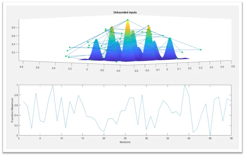
Here we can see optimum value went outside the values of x and y resulting in falling away from stalagmite function. So, we failed to reach the global maxima in this study.
The study time = 6.2355 sec
Step 4: - Study 3 statistical behaviour with bounded input
Here we specify the upper and lower bounds at x and y. we use same program for 2nd study but syntax for ga will change.
[inputs,fopt(k)] = ga(@stalagmite,2,[],[],[],[],[0;0],[1;1]);
OUTPUT
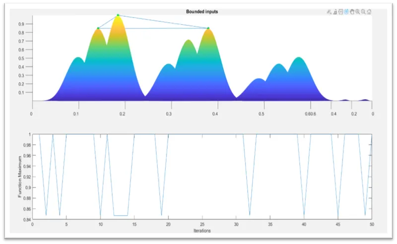
Though the optimum values are within the limit it could not give us the exact maximum values.
The study time = 9.3081 sec
Step 5: - Study 3 statistical behaviour with bounded value.
Here also syntax change as follow because we are changing initial population to 200 so we use optimoption command to change the value of initial iteration.
% Increasing ga iterations
options = optimoptions('ga');
options = optimoptions(options,'PopulationSize',200);
OUTPUT
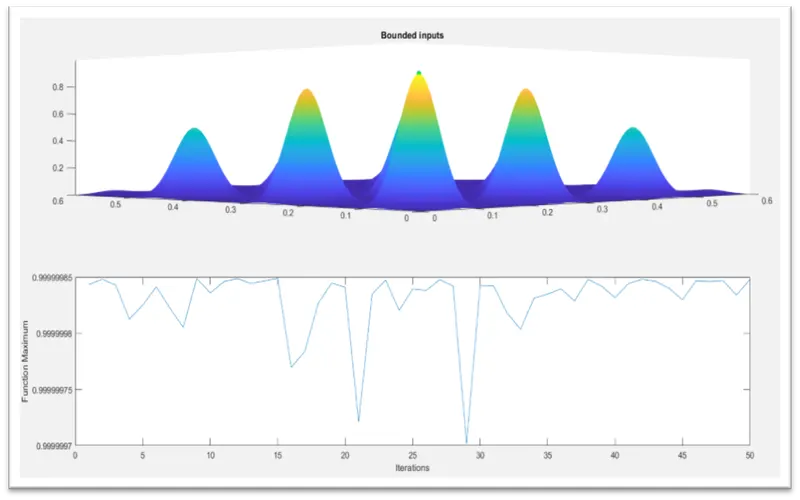
We get global maxima for stalagmite function with help of genetic algorithm but the time require get increase due to increase in no of initial population. When we increase population time also increase. We can’t get same results for every time when we run the code but we get minor change in results. The reason is every time genetic algorithm consider different random value in between consider limit so result change but not major different. Also, when we increase the initial population size, we can increase the accuracy of ga.
The study time = 23.6711 sec
8. CONCLUTION
Genetic algorithm is useful for optimizing the function but result will vary with change in random value we consider. so, we can say that in genetic algorithm we cant get exact value but we get nearby values in result.
A genetic algorithm is a stochastic algorithm, based on random sampling. you will see small differences, even for a function that has a nice global min. So, you can think of the results as all being effectively the same within a tolerance.
If you get different solutions, you still need to accept that for a function that has multiple local maxima, the solver can get trapped in different solutions. Sometimes they may all be equivalent solutions
9. REFERENCES
https://in.mathworks.com/help/gads/genetic-algorithm-options.html
https://in.mathworks.com/help/gads/ga.html?searchHighlight=ga&s_tid=srchtitle_ga_1
https://www.tutorialspoint.com/genetic_algorithms/index.htm
EXTRA WORK
to overcome genetic algorithm problem that using the given programme shown below
clear
close all
clc
%% creating the mesh
x=linspace(0,0.6,150);
y=linspace(0,0.6,150);
[xx,yy]=meshgrid(x,y);
%% for plotting the surface of stalagmite
for i=1:length(xx)
    for j=1:length(yy)
        input_vector(1)=xx(i,j);
        input_vector(2)=yy(i,j);
        f(i,j)=stalagmite(input_vector);
    end
end
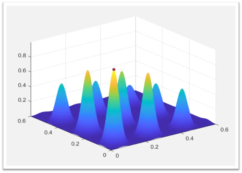
surfc(xx,yy,-f)
shading interp
%% evalutaing the function
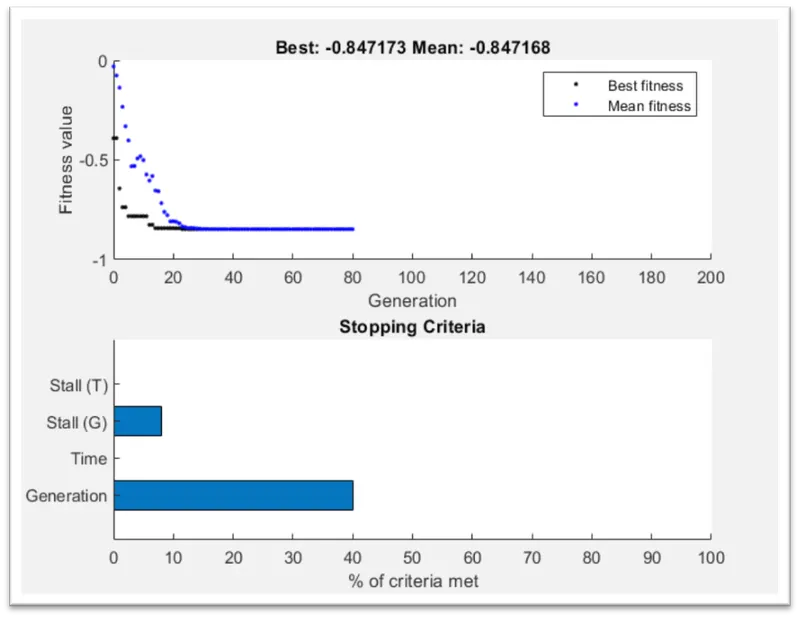
options=optimoptions('ga','PlotFcn',{@gaplotbestf,@gaplotstopping},'populationsize',50);
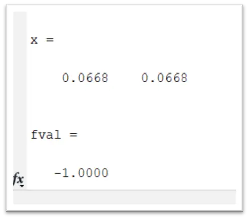
[x,fval]=ga(@stalagmite,2,[],[],[],[],[0;0],[0.6;0.6],[],options)
xopt=x(1);
yopt=x(2);
figure(1)
hold on
plot3(xopt,yopt,-fval,'o','markersize',5,'markerfacecolor','r')
OUTPUT