Simulink

1. AIM: -

To study and analyse the system-level All-Terrain Vehicle model in Simulink and observe results.

2. OBJECTIVE: -

Prepare a technical report explaining the model properties & comments on the results.

3. DESCRIPTION: -

3.1. BAJA All-Terrain Vehicle (ATV)

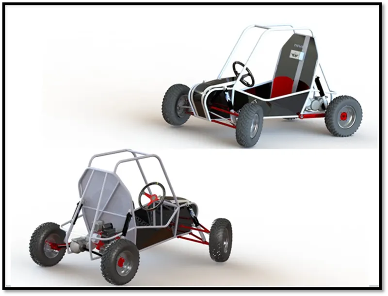
BAJA is basically an ATV competition where students get to design and develop their own ATV keeping in mind various considerations of design as well as safety. An ATV is designed in order to run on various terrains such as soil, Gravel, pebbles, etc.

As per the name an ATV (All-Terrain Vehicle) is designed to run and manoeuvre on different terrains or in other words we can say that an ATV is designed especially for off-roading purpose.

3.2. CONTINUOUS VARIABLE TRANSMISSION: -

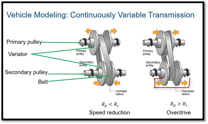
A continuous variable transmission (CVT) is an automatic transmission that can change seamlessly through a continuous range of gear ratios. This contrasts with other transmissions that provide a limited number of gear ratios in fixed steps. The flexibility of a CVT with suitable control may allow the engine to operate at a constant RPM while the vehicle moves at varying speeds. CVTs are used in automobiles, tractors, motor scooters, snowmobiles, bicycles and earthmoving equipment. The most common type of CVT uses two pulleys connected by a belt or chain; however, several other designs have also been used at times.

4. MODEL: - (Simple CVT model)

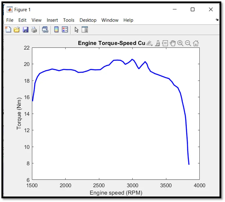
This submission contains a set of models created with Simulink, Simscape, and Simscape Driveline. More specifically, the file contained includes BAJA ATV model with Continuously Variable Transmission (CVT). These models show how to build an ATV with CVT which is mostly used in BAJA competitions. Simscape and Simscape Driveline have been used to complete the system. The engine data used in the model is provided as an image which shows the Engine Speed (RPM) Vs Torque curve. This is an open loop model of CVT.

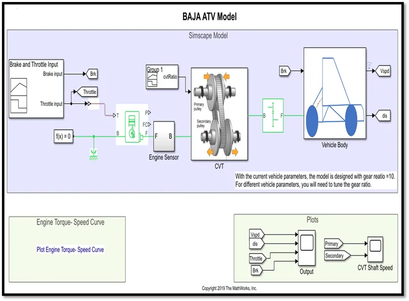
We can see in the above model the input for engine is acceleration (Throttle). Then the engine was connected with CVT and gave rpm input to CVT. The secondary pulley of CVT gave input to simple gear and then simple gear input to vehicle body block in vehicle body subsystem. all output from system is given to output with the help of Goto and from block. Input for engine, CVT and vehicle body from the signal builder block.

In the above model ATV model was made with some inbuild blocks and subsystems as follows,

4.1. MAIN COMPONENTS OF ATV SIMULATION: -

• Generic Engine

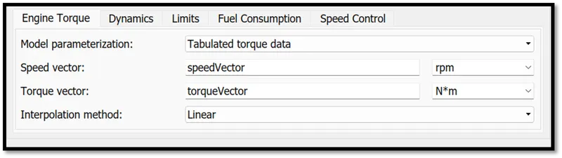
For engine here used generic engine inbuild block. The Generic Engine block represents a general internal combustion engine. This block is a suitable generic engine for spark-ignition and diesel. Speed-power and speed-torque parameterizations are provided. A throttle physical signal input specifies the normalized engine torque. Optional dynamic parameters include crankshaft inertia and response time lag. A physical signal port outputs the engine fuel consumption rate based on the fuel consumption model that you choose. Optional speed and redline controllers prevent engine stalls and enable cruise control.

The throttle input signal T lies between zero and one and specifies the torque demanded from the engine as a fraction of the maximum possible torque.

Connections F and B are mechanical rotational conserving ports associated with the engine crankshaft and engine block, respectively. Connections P and FC are physical signal output ports through which engine power and fuel consumption rate are reported

• Input For Engine (signal builder): -

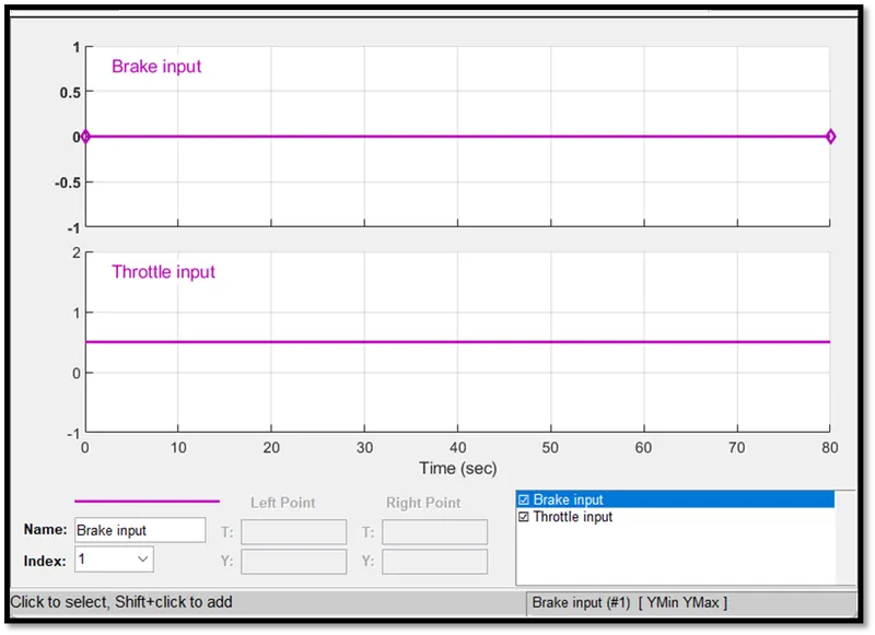
Throttle and breaking these are two inputs for engine, here signal builder is used to give input signal for engine.

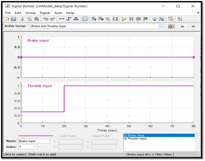
We can observe that currently there is no break input and a constant throttle is provided to the system.

Here the data for engine speed and torque is extracted from the following image of speed and torque data with the help of GRABIT file exchange option. This function extracts the data point from image and saved in workspace to use.

• GRABIT information source: - File Exchange - GRABIT

• Engine sensor: -

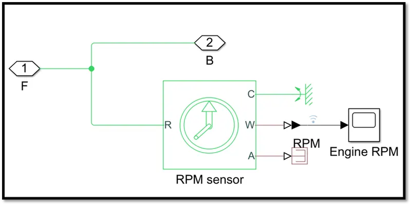
Engine sensor is the Ideal Rotational Motion Sensor block represents an ideal mechanical rotational motion sensor, that is, a device that converts an across variable measured between two mechanical rotational nodes into a control signal proportional to angular velocity or angle. You can specify the initial angular position (offset) as a block parameter.

The sensor is ideal since it does not account for inertia, friction, delays, energy consumption, and so on. Connections R and C are mechanical rotational conserving ports that connect the block to the nodes whose motion is being monitored. Connections W and A are physical signal output ports for velocity and angular displacement, respectively.

The block positive direction is from port R to port C. This means that the velocity is measured as ω = ωR – ωC, where ωR, ωC are the absolute angular velocities at ports R and C, respectively

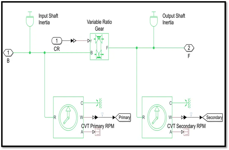
• CVT Subsystem

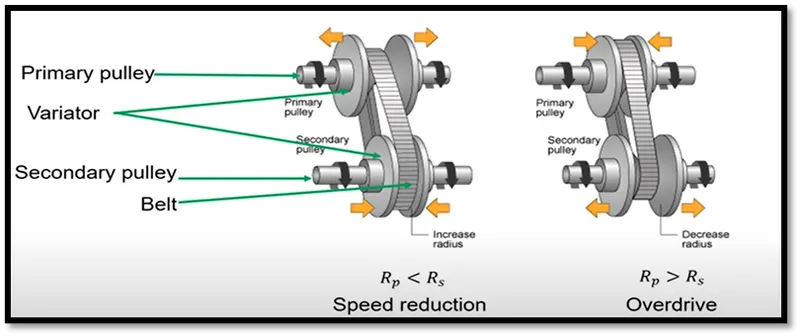
here we are using gear reduction drive of CVT which is lower speed instead of overdrive you can see the difference in following image.

here we are using gear reduction drive of CVT which is lower speed instead of overdrive you can see the difference in following image.

For CVT there is not any block so here sub system for that was created. Which contains the following blocks,

1. Go to: - Send signals to from blocks that have the specified tag. If tag visibility is 'scoped', then a Goto Tag Visibility block must be used to define the visibility of the tag. The block icon displays the selected tag name (local tags are enclosed in brackets, [], and scoped tag names are enclosed in braces, {}).
2. Inport: - Provide an input port for a subsystem or model.
3. Inertia: - The block represents an ideal mechanical rotational inertia.
4. PMC_port: - Physical Modelling Connection Port block for subsystems.
5. Variable ratio gear transmission: - Represents a variable ratio gearbox such as implemented by mechanical belt CVT, electric, or hydraulic transmissions. The physical signal input r defines the ratio of input to output angular shaft velocities. Connections B (base) and F (follower) are mechanical rotational conserving ports. Specify the relation between base and follower rotation directions with the Output shaft rotates parameter.
6. Ps terminator: - Use this block to terminate physical signal outputs. Unconnected physical signal output ports do not generate warnings, but connection to a PS Terminator can be used to indicate that the signal was not inadvertently left unconnected.
7. Mechanical Rotational Reference: - This block represents a mechanical rotational reference point, that is, a frame or a ground. Use it to connect mechanical rotational ports that are rigidly affixed to the frame (ground).
8. PS-Simulink Converter: - Converts the input Physical Signal to a Simulink output signal.
9. The unit expression in 'Output signal unit' parameter must match or be commensurate with the unit of the Physical Signal and determines the conversion from the Physical Signal to the Simulink output signal.

4.2. Input for CVT: -

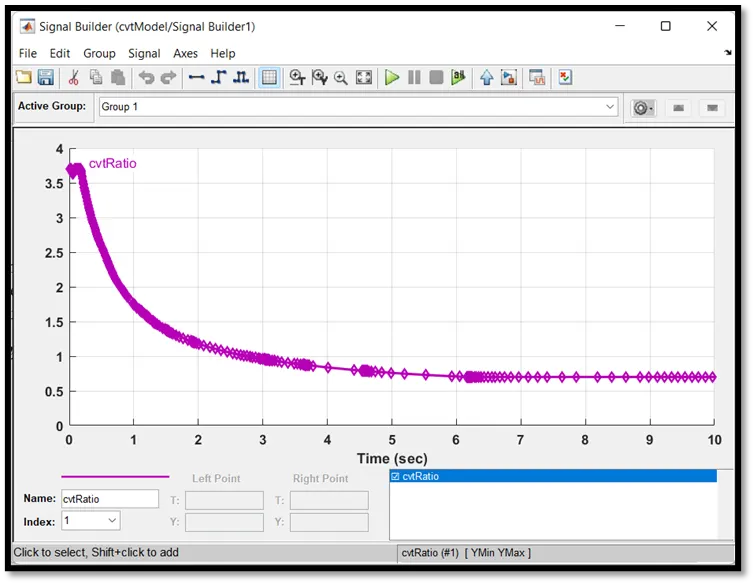
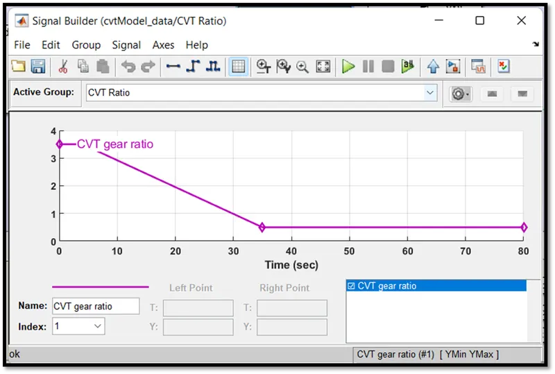
The input for CVT subsystem is CVT ratio and engine rpm. Engine rpm we discuss above and CVT ratio is given by signal builder.

• Simple gear: -

Represents a fixed-ratio gear or gear box. No inertia or compliance is modelled in this block. You can optionally include gear meshing, backlash, and viscous bearing losses. Connections B (base) and F (follower) are mechanical rotational conserving ports. Specify the relation between base and follower rotation directions with the Output shaft rotates parameter. Optionally include thermal effects and expose thermal conserving port H by setting Friction model to a temperature-dependent setting.

With the current vehicle parameters, the model is designed with gear ratio =10. For different vehicle parameters, you will need to tune the gear ratio.

To connect the engine and CVT we need speed reduction so we add simple gear block.

• Vehicle body Subsystem

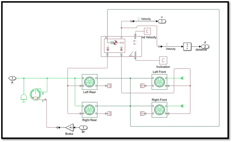
The above model is a graphical representation of vehicle body(frame) and wheel.

For the vehicle body there is a block but for input connect tire and brake to block so here subsystem was created. Which contains the following blocks,

Vehicle body: -Represents a two-axle vehicle body in longitudinal motion. The block accounts for body mass, aerodynamic drag, road incline, and weight distribution between axles due to acceleration and road profile. The vehicle can have the same or a different number of wheels on each axle. Optionally include pitch and suspension dynamics or additional variable mass and inertia. The vehicle does not move vertically relative to the ground.

Connection H is the mechanical translational conserving port associated with the horizontal motion of the vehicle body. The resulting traction motion developed by tires should be connected to this port. Connections V, NF, and NR are physical signal output ports for vehicle velocity and front and rear normal wheel forces, respectively. Wheel forces are considered positive if acting downwards. Connections W and beta are physical signal input ports corresponding to headwind speed and road inclination angle, respectively. If variable mass is modelled, the physical signal input ports CG and M are exposed. CG accepts a two- element vector representing the x and y distance offsets from vehicle CG to additional load mass CG. M represents the additional mass. If both variable mass and pitch dynamics are included, the physical signal port J accepts the inertia of the additional mass about its own CG.

Tire (Magic Formula): -

Represents the longitudinal behaviour of a highway tire characterized by the tire Magic Formula. The block is built from Tire-Road Interaction (Magic Formula) and Simscape Foundation Library Wheel and Axle blocks. Optionally, the effects of tire inertia, stiffness, and damping can be included.

Connection A is the mechanical rotational conserving port for the wheel axle. Connection H is the mechanical translational conserving port for the wheel hub through which the thrust developed by the tire is applied to the vehicle. Connection N is a physical signal input port that applies the normal force acting on the tire. The force is considered positive if it acts downwards. Connection S is a physical signal output port that reports the tire slip. Optionally expose physical signal port M by setting Parameterize by to Physical signal Magic Formula coefficients. Physical signal port M accepts a four-element vector corresponding to the B, C, D, and E Magic Formula coefficients.

Double shoe break: -

Represents a brake arranged as two pivoted rigid shoes symmetrically installed inside or outside a drum and operated by one actuator. The actuator force causes the shoes to exert a friction torque on a shaft connected to the drum.

Connection S is a conserving rotational terminal associated with the drum shaft. Connection F is a physical signal port representing the force input to the actuator. Positive force creates friction torque that resists shaft rotation. Optionally include thermal effects and expose thermal conserving port H by setting Thermal port to Model.

4.3. OUTPUT RESULTS: -

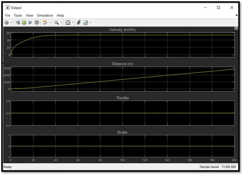
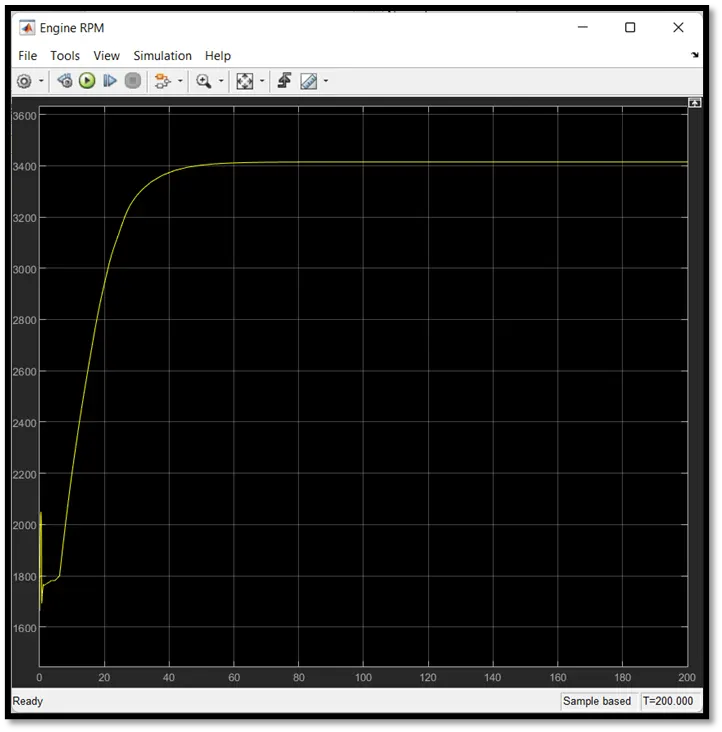
In the above graph we can see that the velocity increases over time to 40 sec but after that it will constant. We cover a 3km distance with 0.5 throttled input and no brake applied.

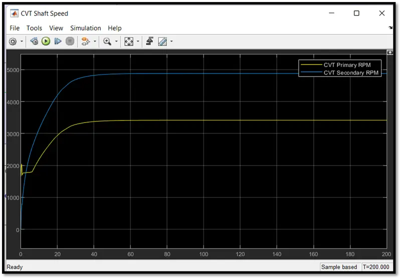
Here we can see that the secondary pulley rpm is greater than primary pulley because when we accelerate the vehicle the primary pulley will expand and secondary pulley will extract this process is nothing but speed reduction.

5. MODEL: - (Simple CVT Model with Dashboard)

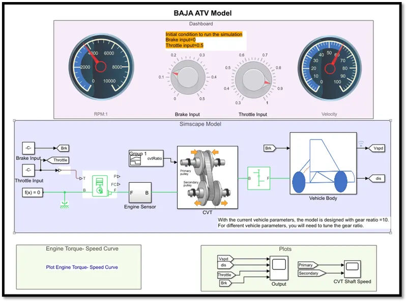
In this model we are used to the same model but with different input in running time for actual simulation with help of different block other parameters are all same. To give input dashboard knobs are used which are connected with constant block which provide input in running time. We gave infinite time for running so we can change the speed and observe the results. This is an open loop model of CVT.

5.1. BLOCKS USED: -

• Circular gauge: - (Rpm, Velocity)

Display an input value on a customized gauge. Here we connect this block to rpm engine and velocity of body.

• Circular knob: - (Brake input, Throttle input)

Set a value to tune parameters or variables. Here we connect the block to input constant block which is brake and Throttle.

5.2. OUTPUT RESULTS: -

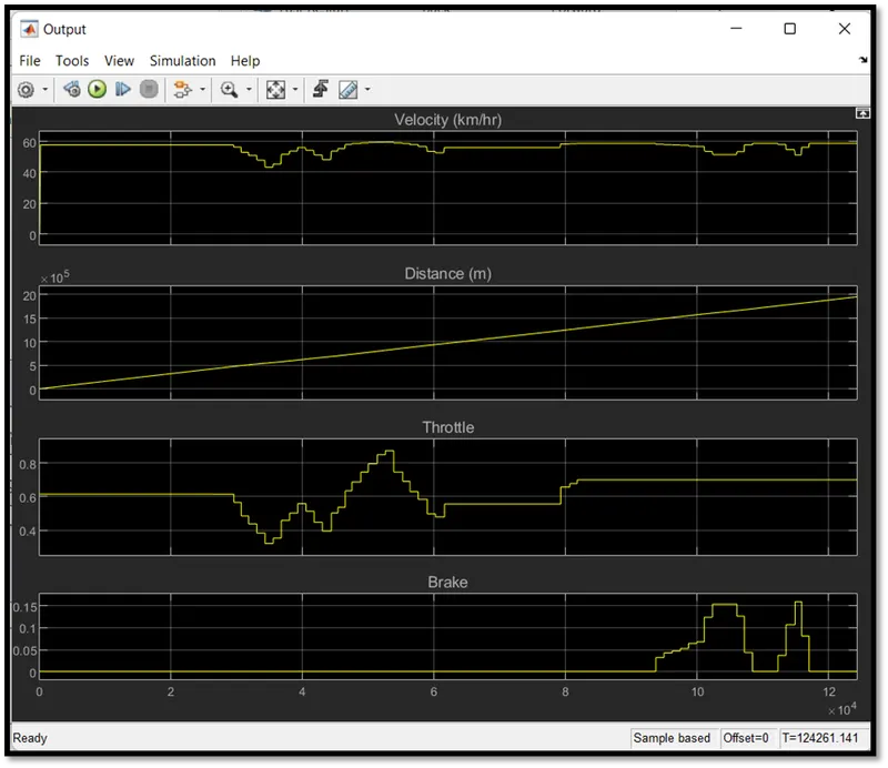
Here we can see that the response of model to the throttle input and brake input. When we start the simulation the velocity at 60km/hr then we reduce throttle gradually then velocity also decreased. When we apply a brake then also, we can see that the velocity decreased so we can say that the vehicle speed totally depends on throttle and brake input.

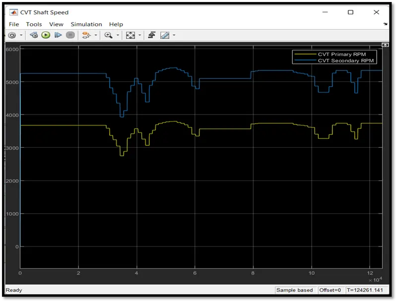
Here we can see that the velocity and CVT RPM graph are identical and primary pulley rpm is less than the secondary pulley rpm because we are using speed reduction drive for CVT.

6. MODEL: - (simple CVT Model Data Extraction)

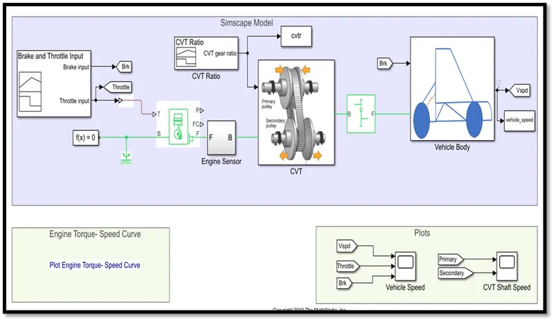
Here we are only changing our input data for more visualization.

6.1. New input: -

6.2. Output for new results: -

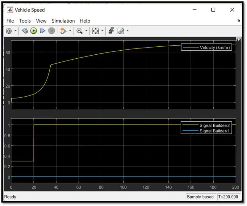
Here we can see that we give input throttle and brake and velocity graph also responding according to input given.

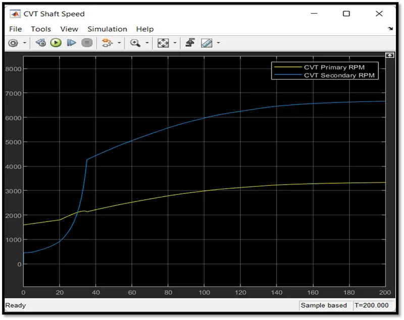
Here we can observe till 30 sec the secondary pulley RPM is less than secondary because input we gave sudden acceleration after 20 second then constant to 1. So, after 30 again the secondary pully rpm increased and primary pully rpm decreased. Hence, we can say that till 30sec the CVT is in overdrive and after 30 sec in speed reduction drive.

Here we used a simple model to extract the CVR ratio data.

6.3. Code to extract data: -

%% Load and simulate the model
cvtModel_data
sim('cvtModel_data')

%% Visualize the lookup table 
plot(vehicle_speed,cvtr,'r','LineWidth',2)
xlabel ('Vehicle Speed (km/hr)')
ylabel ('CVT Ratio')
title ('Lookup Table Visualization')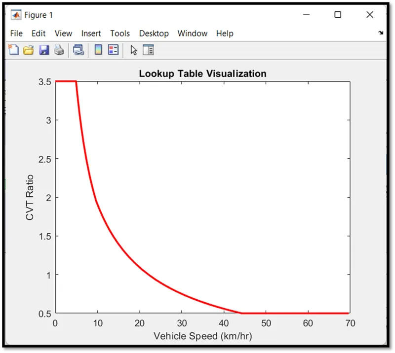

Here we get the CVT ratio to Vehicle Speed plot for lookup table input.

7. MODEL: - (Mapped CVT Model)

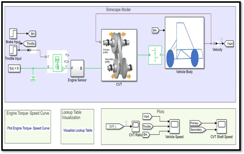
Here we are used lookup table for input the CVT ratio with the help of lookup table visualization and input with step block. This is a close loop model of CVT.

7.1. Blocks used in model: -

Blocks used in model: -

Lookup table: - A lookup table is an array of data that maps input values to output values, thereby approximating a mathematical function. Given a set of input values, a lookup operation retrieves the corresponding output values from the table. If the lookup table does not explicitly define the input values, Simulink can estimate an output value using interpolation, extrapolation, or rounding, where:

• An interpolation is a process for estimating values that lie between known data points.
• An extrapolation is a process for estimating values that lie beyond the range of known data points.
• A rounding is a process for approximating a value by altering its digits according to a known rule.

A lookup table block uses an array of data to map input values to output values, approximating a mathematical function. Given input values, Simulink performs a “lookup” operation to retrieve the corresponding output values from the table. If the lookup table does not define the input values, the block estimates the output values based on nearby table values.

Since table lookups and simple estimations can be faster than mathematical function evaluations, using lookup table blocks might result in speed gains when simulating a model. Consider using lookup tables in lieu of mathematical function evaluations when:

• An analytical expression is expensive to compute.
• No analytical expression exists, but the relationship has been determined empirically.

PS lookup table: -

This block represents a physical signal converter whose input-output relationship is specified by a lookup table. The table grid must be in strictly ascending or strictly descending order, but the spacing can be nonuniform. Right-click on the block and select Foundation Library > Plot Table to visualize the table data based on the selected interpolation and extrapolation methods.

This block does not propagate physical signal units and will be removed in a future release. Use the Upgrade Advisor to update this block to the latest version.

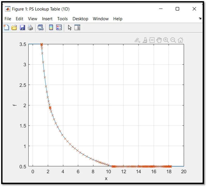
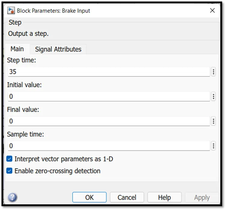
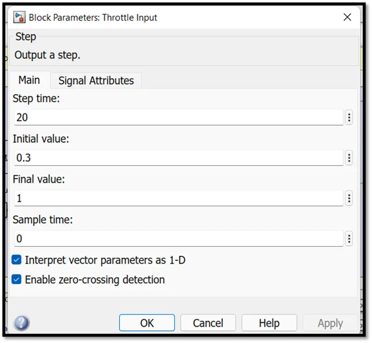
Input for step block: -

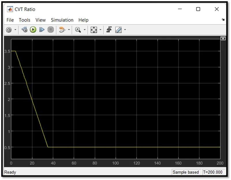
7.3. Input for CVT ratio: -

7.4. Output results: -

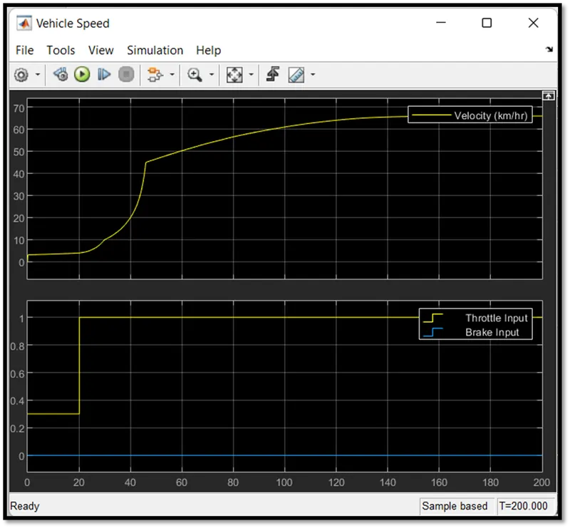
Here we can see that we give input throttle and brake and velocity graph also responding according to input given.

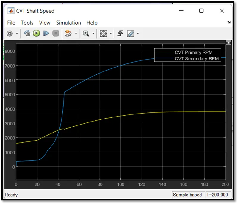
Here we can observe till 40 sec the secondary pulley RPM is less than secondary because input we gave sudden acceleration after 20 second then constant to 1. So, after 40sec again the secondary pully rpm increased and primary pully rpm decreased. Hence, we can say that up to 40sec the CVT is in overdrive and after 40 sec in speed reduction drive.

8. MODEL: - (Mapped CVT Model with dashboard)

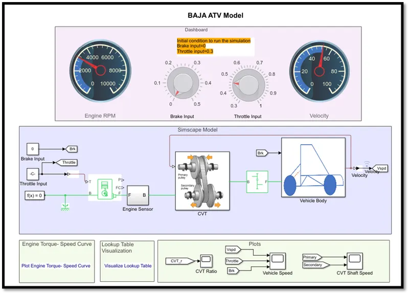
Here we are used lookup table for input the CVT ratio and input with control knob as above dashboard model. This is a close loop model of CVT.

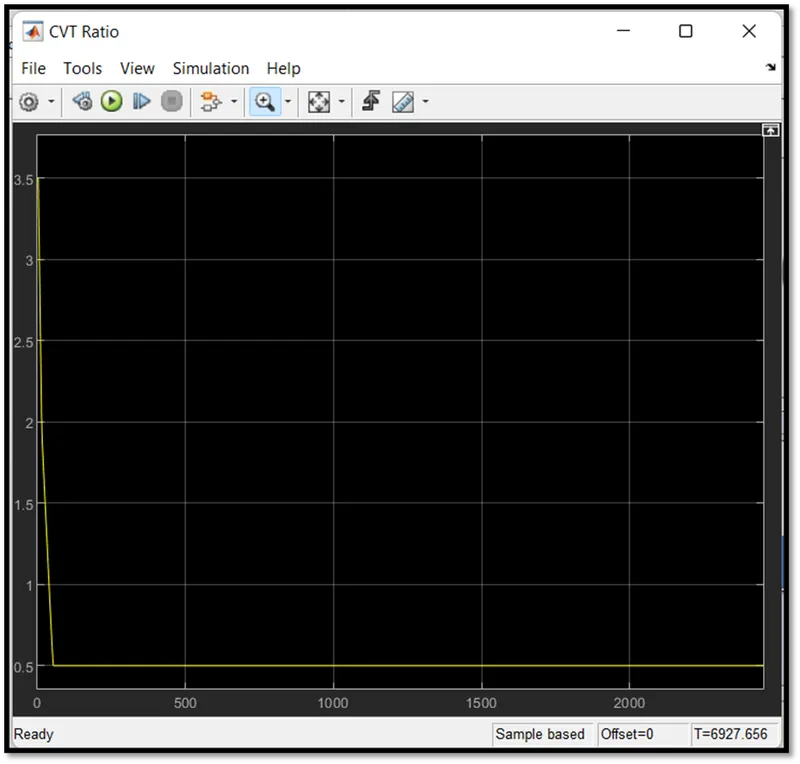
8.1. Input for CVT Ratio: -

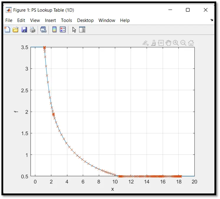
8.3 Output results: -

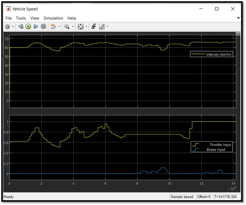
In the above figure we can see that velocity follows the same path as the input which is throttle input and brake input.

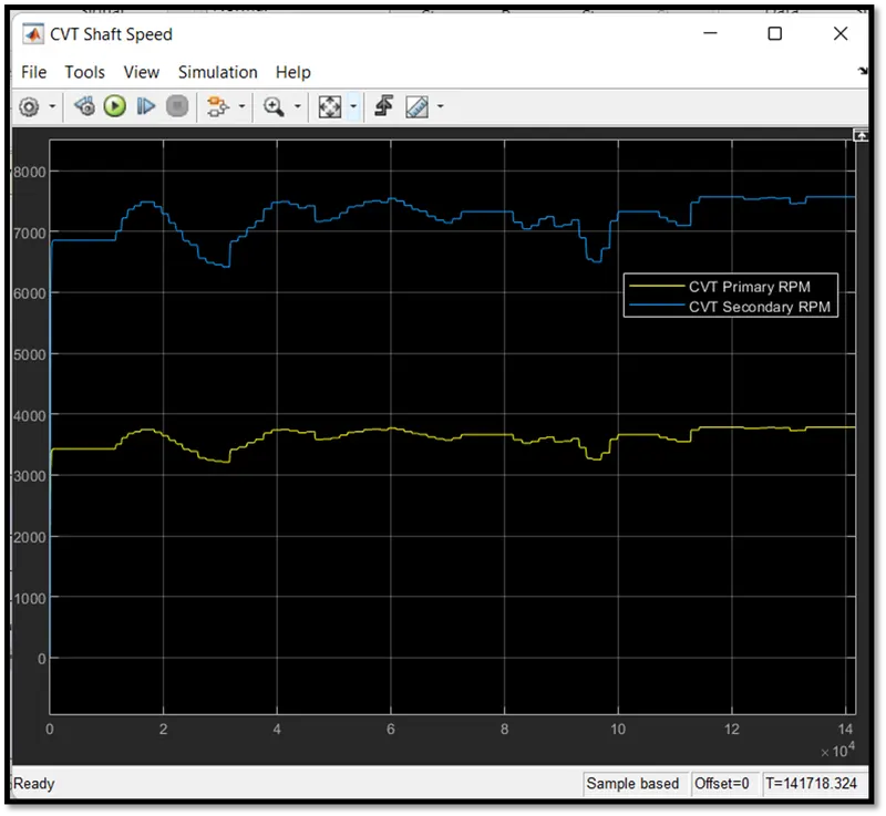
Here we can see that the velocity and CVT RPM graph are identical and primary pulley rpm is less than the secondary pulley rpm because we are using speed reduction drive for CVT.

9. CONCLUSION: -

We can conclude that we have successfully simulated the Baja All-Terrain Vehicle with different methods like open loop model and close loop model. We got satisfactory results for the simulation. We can use this model to simulate actual data for SAE competition.

10. References: -

• https://in.mathworks.com/matlabcentral/fileexchange/70576-baja-all-terrain-vehicle-atv-model
• https://in.mathworks.com/support.html?s_tid=gn_supp
• https://youtu.be/gOFweQcz0XI

11. MODEL FILE: -

• ATV Model Files