MATLAB PROGRAM FOR FLOW OVER BICYCLE
Calculate Drag force on a bicycle.
Aim: - Write a Matlab program to calculate drag force against a cyclist
Objective: -
- Write a program to plot Velocity vs Drag force.
- Write a program to plot Drag Co-efficient vs Drag force.
Formula
Fd = 1/2*ρ*V^2*A*Cd
Were,
Fd = drag force (N)
Cd = drag coefficient
ρ = density of fluid (1.2 kg/m3 for air at NTP)
v = flow velocity (m/s)
A = characteristic frontal area of the body (m2)
Input
Rho = 1.2
A = 0.1
V = 1 (1:50)
Cd = 0.8 (1:50)
Description
- Drag force is a resistive force acting on the body in a particular direction by fluid(air) on the frontal area of the cyclist.
- The drag coefficient is a function of several parameters like the shape of the body, Reynolds Number for the flow, Froude number, Mach Number, and Roughness of the Surface. It depends on the frontal area.
- The characteristic frontal area - A - depends on the body.
Different position of a cyclist
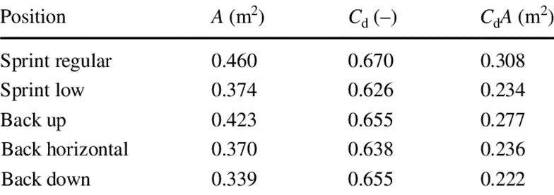
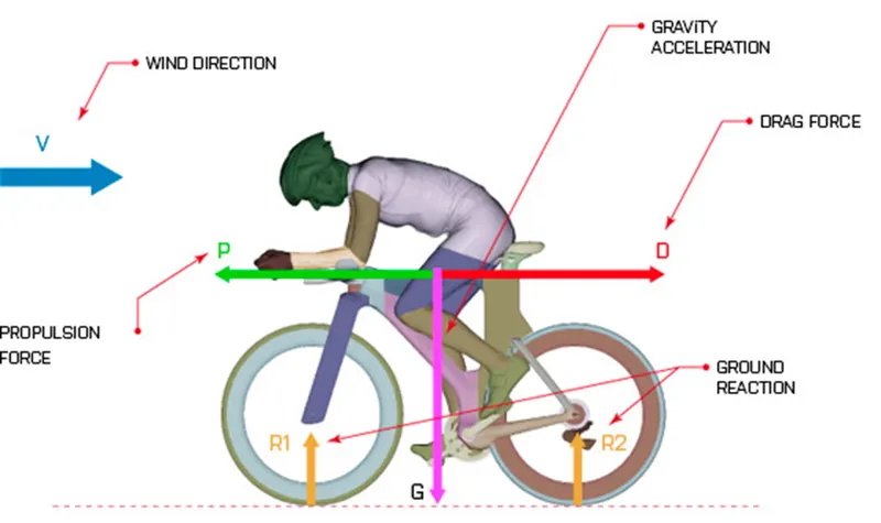
Here we can see when we are riding bicycle at different velocity the frontal area (A) is constant but the Drag coefficient is different for different frontal area. Drag force is directly depend on frontal area and velocity of cyclist. It means when velocity is increased simultaneously drag force also increase, same as when frontal area is change simultaneously drag coefficient and drag force also changes.
MATLAB program
1. Program to plot a graph for Velocity vs Drag force
% A program to calculate drag force on a bicycle
clearvars
close all
clc
% Input
% Drag coefficient
C_d = 0.8;
% Area m^2
A = 0.1;
% Density Kg/ m^3
rho = 1.2;
% Velocity
V = (1:50);
% Drag force kgm/s^2
Drag_force = rho*A*V.^2*C_d.*0.5;
plot(V, Drag_force,'color','r');
xlabel('Velocity');
ylabel('Drag force');
title('Velocity vs Drag force');
grid on
Command Window results
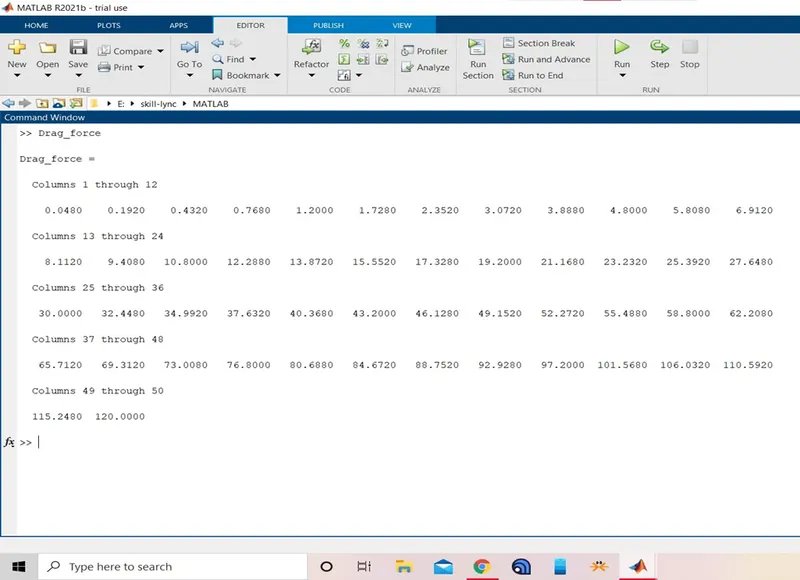
Graph: - Velocity vs Drag force
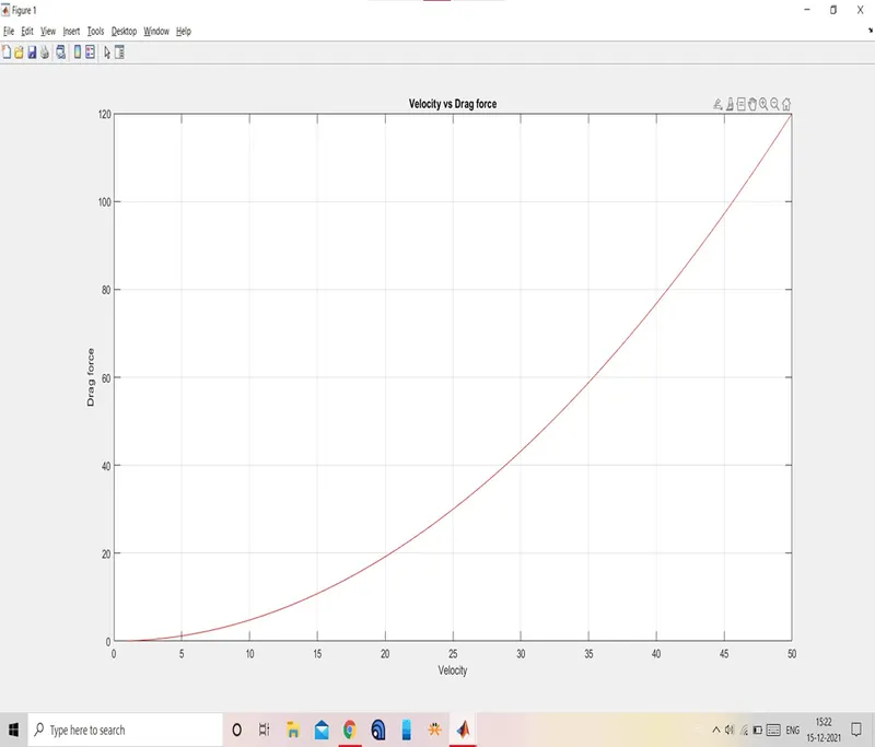
Conclusion: -
From the above results, we can conclude that Drag force is directly proportional to velocity square.
2. Program to plot a graph for Drag coefficient vs Drag force
clearvars
close all
clc
% Input
% Drag coefficient
C_d = [0.67 0.62 0.65 0.63 0.65];
label = {'Sprint regular','Sprint low','Back up', 'back horizontal','back down'};
% Area m^2
A = 1;
% Density Kg/ m^3
rho = 1.2;
% Velocity
V = 0.25;
% Drag force kgm/s^2
drag_force = rho*A.*V^2*C_d.*0.5;
plot (C_d, drag_force,'marker','s','markerfacecolor','r');
text(C_d,drag_force,label);
xlabel('C_d');
ylabel('Drag force');
title ('Drag coefficient vs Drag force');
grid on
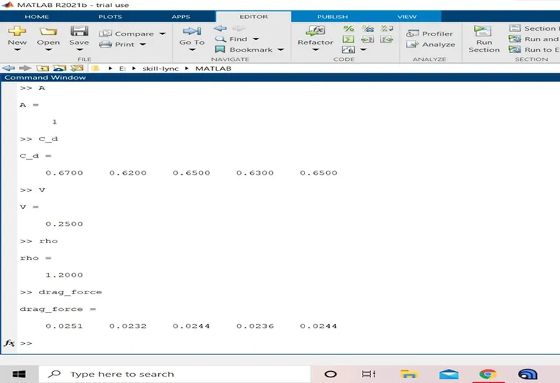
Command Window
Graph: - Drag coefficient vs Drag force
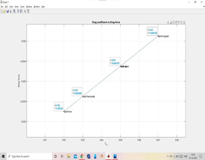
Conclusion: -
From the above results, we can conclude that the Drag coefficient is directly proportional to the Drag force.
Hence, we can conclude that the drag force is as low as possible so we can get better efficiency.