Project 2 - Rankine cycle Simulator
OBJECTIVE:
To create a Rankine Cycle Simulator using MATLAB and calculate its state-points.
THEORY:
RANKINE CYCLE:
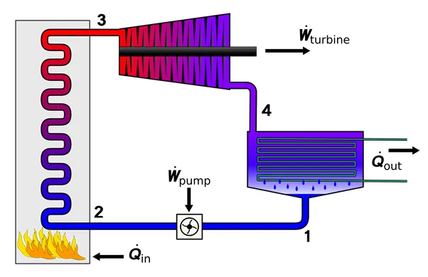
The Rankine Cycle is a mechanical cycle commonly used in power plants to convert the pressure energy of steam into mechanical energy through steam turbines. Major components include a Rotating steam turbine, a boiler pump, a stationary condenser and a boiler.
In this mechanism, a fuel is used to produce heat within a boiler, converting water into steam which expands through a turbine producing useful work. This process was developed by a Scotting Engineer William J.N. Rankine in 1859. It’s a thermodynamic cycle that converts heat into mechanical energy, which usually gets transformed into electricity by electrical generation.
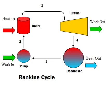
The efficiency of the Rankine Cycle is limited by the High Heat of Vaporization of the fluid. The fluid must be cycled through and reused constantly. So, water is the most practical fluid for this cycle.
As the water condenses in the condenser, Waste Heat is given off in the form of Water Vapour. This waste heat is necessary for any thermodynamic cycle. Due to this condensation step, the pressure at the turbine outlet is lowered. This means the pump requires less work to compress the water, Resulting in Higher Overall Efficiency.
OPERATION OF RANKINE CYCLE:
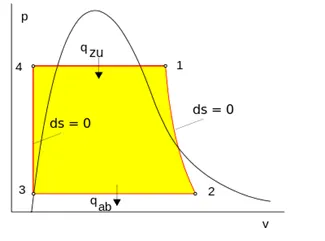
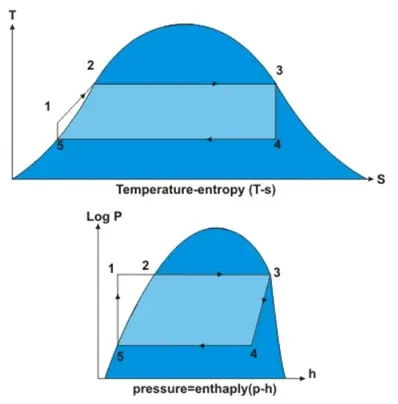
- 1-2-3 – ISOBARIC HEAT TRANSFER: (Constant pressure heat addition in boiler)
The high-pressure liquid enters the boiler from the Feed Pump (1) and is heated to the saturation temperature (2).
Further addition of heat caused the evaporation of liquid until it is fully converted to saturated steam (3).
- 3-4 – ISENTROPIC EXPANSION: (In a turbine)
The vapour is expanded in the turbine, thus producing work that may be converted to electricity. In practice, the expansion is limited by the temperature of the cooling medium and by the erosion of the turbine blades by liquid entrainment in the vapour stream as the process moves further into 2 – phase region. Exit vapour qualities should be >90%.
- 4-5 – ISOBARIC HEAT REJECTION: (Constant heat rejection or Constant Pressure Heat Rejection in a condenser)
The vapour – liquid mixture leaving the turbine (4) is condensed at low pressure, usually in a surface condenser using cooling water. In well-designed and maintained condensers, the pressure of the vapour is well below atmospheric pressure, approaching the saturation pressure of the operating fluid at the cooling water temperature.
- 5-1 – ISENTROPIC COMPRESSION: (In a pump)
The pressure of the condensate is raised in the feed pump. Because of the low specific volume of the liquids, the pump work is relatively small and often neglected in thermodynamic calculations.
%% Program to Simulate the Rankine Cycle

% Rankine Cycle - It's a mechanical cycle commonly used in power plants to
% convert the pressure energy of the steam into mechanical energy through
% steam turbines.
% Major components include ROTATING STEAM TURBINE, A BOLIER PUMP, A
% STATIONARY CONDENSER & A BOILER.

% EFFICIENCY -  The Efficiency of the Rankine Cycle is limited by the High
% Heat of Vaporization by the fluid. The fluid must be cycled through and
% must be reused constantly. So, Water is the most practical fluid for this
% cycle. Because, as the water condenses in the condenser, Waste Heat is
% given off in the form of Water Vapour. This waste heat is necessarry in
% any thermodynamic cycle.

% Rankine cycle comprises following processes -
% 1. 1-2-3 ISOBARIC HEAT TRANSFER (constant pressure heat addition in
%          boiler)

% 2. 3-4   ISENTROPIC EXPANSION (in a turbine)

% 3. 4-5   ISOBARIC HEAT REJECTION (constant heat rejection or constant
%          pressure heat rejection in a condenser)

% 4. 5-1   ISENTROPIC COMPRESSION (in a pump)

clear all
close all
clc

%% Required Inputs
Temperature_1 = input ('Value of temperature at turbine inlet = C\n');    % Turbine in-let Temperature in C
Pressure_1 = input ('\nValue of pressure at turbine inlet = bar\n');        % Turbine in-let pressure in bar
Pressure_2 = input ('\nValue of pressure at turbine outlet = bar\n');      % Turbine out-let pressure in bar ( Condenser in-let Pressure)

%% State Variables at STATE POINT - 1
H1 = XSteam ('h_pT', Pressure_1, Temperature_1);        % Turbine In-let Enthalpy [kJ/kg]
Volume_1 = XSteam ('v_pT', Pressure_1, Temperature_1);  % Turbine In-let Volume [m^3/kg]
S1 = XSteam ('s_pT', Pressure_1, Temperature_1);        % Turbine In-let Entropy [kJ/kg K]

%% State Variables at STATE POINT - 2
S2 = S1;                                                           % Conderser In-let Entropy [kJ/kg K]
H2 = XSteam('h_px', Pressure_2, XSteam ('x_ps', Pressure_2, S2));  % Conderser In-let Enthalpy [kJ/kg]
Temperature_2 = XSteam('T_ps', Pressure_2, S2);                    % Conderser In-let Temperature [degree C]
Volume_2 = XSteam('v_ps', Pressure_2, S2);                         % Conderser In-let Specific Volume [m^3/kg]

%% State Variables at STATE POINT - 3
Pressure_3 = Pressure_2;                            % Pump In-let Pressure [bar]
Temperature_3 = XSteam ('Tsat_p', Pressure_3);      % Pump In-let Temperature [degree C]
H3 = XSteam ('hL_p', Pressure_3);                   % Pump In-let Enthalpy [kJ/kg]
S3 = XSteam ('sL_p', Pressure_3);                   % Pump In-let Entropy [kJ/kg K]
Volume_3 = XSteam ('vL_p', Pressure_3);             % Pump In-let Specific Volume [m^3/kg]

%% State Variables at STATE POINT - 4
S4 = S3;                                          % Boiler In-let Entropy [kJ/kg K]
Pressure_4 = Pressure_1;                          % Boiler In-let Pressure [bar]
H4 = XSteam ('h_ps', Pressure_4, S4);             % Boiler In-let Enthalpy [kJ/kg]
Temperature_4 = XSteam ('T_ps', Pressure_4, S4);  % Boiler In-let Temperature [degree C]
Volume_4 = XSteam ('v_ps', Pressure_4, S4);       % Boiler In-let Specific Volume [m^3/kg]

%% Calculating the Temperature, Entropy and Enthalpy at the Vapour & Liquid phase line for plotting

Temperature_6 = XSteam ('Tsat_p', Pressure_1);
S5 = XSteam ('sL_p', Pressure_1);
S6 = XSteam ('sV_p', Pressure_1);
H5 = XSteam ('hL_p', Pressure_1);
H6 = XSteam ('hV_p', Pressure_1);
Temperature_5 = Temperature_6;

%% Plotting the Saturation Curve

Temperature = linspace (1, 375, 1000);

for i = 1 : length (Temperature)
    sf (i) = XSteam ('sL_T', Temperature (i));
    sg (i) = XSteam ('sV_T', Temperature (i));
    hf (i) = XSteam ('hL_T', Temperature (i));
    hg (i) = XSteam ('hV_T', Temperature (i));

end
%% Plotting T vs S path for Ideal Rankine cycle

figure (1)
hold on
plot (sf, Temperature, 'k', 'linewidth', 1.5);
plot (sg, Temperature, 'k', 'linewidth', 1.5);
plot ([S1 S2], [Temperature_1 Temperature_2], 'color', [0 0.4470 0.7410], 'linewidth', 3);
plot ([S2 S3], [Temperature_2 Temperature_3], 'color', [0.8500 0.3250 0.0980], 'linewidth', 3);
plot ([S3 S4], [Temperature_3 Temperature_4], 'color', [0.9290 0.6940 0.1250], 'linewidth', 3);
plot ([S4 S5], [Temperature_4 Temperature_5], 'color', [0.4940 0.1840 0.5560], 'linewidth', 3);
plot ([S5 S6], [Temperature_5 Temperature_6], 'color', [0.4660 0.6740 0.1880], 'linewidth', 3);

Temp_Range = linspace (Temperature_4, Temperature_1, 100);

for i = 1 : length (Temp_Range)
    S_Range (i) = XSteam ('s_pT', Pressure_1, Temp_Range(i));
    H_Range23 (i) = XSteam ('h_ps', Pressure_1, S_Range(i));
    H_Range41 (i) = XSteam ('h_ps', Pressure_2, S_Range(i));
end

plot (S_Range, Temp_Range, 'color', 'g', 'linewidth', 1.8);
legend ('Reversible Adiabatic Expansion', 'Constant Pressure Heat Rejection', 'Reversible Isentropic Compression', 'Constant Pressure Heat Addtion');

%% Plotting H vs S path for Ideal Rankine cycle

figure(2)
hold on
plot (sf, hf, 'k', 'linewidth', 1)
plot (sg, hg, 'k', 'linewidth', 1)
plot ([S1 S2], [H1 H2], 'color', [0 0.4470 0.7410], 'linewidth', 3);
plot (S_Range, H_Range23, 'color', [0.8500 0.3250 0.0980], 'linewidth', 3);
plot ([S3 S4], [H3 H4], 'color', [0.9290 0.6940 0.1250], 'linewidth',3);
plot (S_Range, H_Range41, 'color', [0.4940 0.1840 0.5560], 'linewidth',3);
legend ('Reversible Adiabatic Expansion', 'Constant Pressure Heat Rejection', 'Reversible Isentropic Compression', 'Constant Pressure Heat Addtion');

%% Plotting H vs S path for Ideal Rankine cycle

figure (3)
hold on
Press_Range12 = linspace (Pressure_2, Pressure_1, 100);

for i = 1 : length (Press_Range12)
    V_Range12 (i) = XSteam ('v_ps', Press_Range12 (i), S1);
    V_Range34 (i) = XSteam ('v_ps', Press_Range12 (i), S3);
end

plot (V_Range12, Press_Range12, 'color', [0 0.4470 0.7410], 'linewidth', 3);
plot ([Volume_2 Volume_3], [Pressure_2 Pressure_3], 'color', [0.8500 0.3250 0.0980], 'linewidth', 3);
plot (V_Range34, Press_Range12, 'color', [0.9290 0.6940 0.1250], 'linewidth', 3);
plot ([Volume_4 Volume_1], [Pressure_4 Pressure_1], 'color', [0.4940 0.1840 0.5560], 'linewidth', 3);
legend ('Reversible Adiabatic Expansion', 'Constant Pressure HeatRejection', 'Reversible Isentropic Compression', 'Constant Pressure Heat Addtion');

%% Ploting T vs S Diagram for Water

Temp_Range = linspace (0, 374.15, 500);       % Temperature from 0 to critical point of water [degree C]
figure(1)
hold on

for i = 1 : length (Temp_Range)
    plot (XSteam ('sL_t', Temp_Range (i)), Temp_Range (i), '-.', 'color', 'b')
    plot (XSteam ('sV_t', Temp_Range (i)), Temp_Range (i), '-.', 'color', 'b')
end

%% Ploting h vs S Diagram for Water

figure(2)
hold on

for i = 1 : length (Temp_Range)
    plot (XSteam ('sL_t', Temp_Range (i)), XSteam ('hL_t', Temp_Range (i)), '-', 'color', 'b')
    plot (XSteam ('sV_t', Temp_Range (i)), XSteam ('hV_t', Temp_Range (i)), '-', 'color', 'b')
end

%% Ploting P vs V Diagram for Water

figure(3)
hold on
grid on

for i = 1 : length (Temp_Range)
    plot (XSteam ('vL_t', Temp_Range (i)), XSteam ('p_hs', XSteam ('hL_t', Temp_Range (i)), XSteam ('sL_t', Temp_Range (i))), '--', 'color', 'b')
    plot (XSteam ('vV_t', Temp_Range (i)), XSteam ('p_hs', XSteam ('hV_t', Temp_Range (i)), XSteam ('sV_t', Temp_Range (i))), '--', 'color', 'b')
end

%% Ploting Diagram state points for Ideal Rankine cycle in T vs S

figure(1)
hold on

plot (S1, Temperature_1, 'ko');
plot (S2, Temperature_2, 'ko');
plot (S3, Temperature_3, 'ko');
plot (S4, Temperature_4, 'ko');

grid on

title ('T vs S Diagram of RANKINE CYCLE');
xlabel ('TEMPERATURE [degree C]');
ylabel ('SPECIFIC ENTROPY [kJ/kg K]');

%% Ploting Diagram state points for Ideal Rankine cycle in H vs S

figure(2)
hold on
plot (S1, H1, 'ko');
plot (S2, H2, 'ko');
plot (S3, H3, 'ko');
plot (S4, H4, 'ko');

grid on

title ('H vs S Diagram of RANKINE CYCLE');
xlabel ('ENTHALPY [kJ/kg]');
ylabel('SPECIFIC ENTROPY  in [kJ/kg K]')

%% Ploting Diagram state points for Ideal Rankine cycle in p vs v

figure(3)
hold on
plot (Volume_1, Pressure_1, 'ko');
plot (Volume_2, Pressure_2, 'ko');
plot (Volume_3, Pressure_3, 'ko');
plot (Volume_4, Pressure_4, 'ko');

grid on

title ('P vs V Diagram of RANKINE CYCLE');
xlabel('SPECIFIC VOLUME [m^3/kg]');
ylabel('PRESSURE [bar]');

%% Calculating Work and Efficiency

WORK_TURBINE = H1 - H2;                         % Work transferred from the working fluid (kJ/kg)
Q_CONDENSER = H2 - H3;                          % heat rejected from the working fluid (kJ/kg)
WORK_PUMP = H4 - H3;                            % work transferred into the working fluid (kJ/kg)
Q_BOILER = H1 - H4;                             % heat transferred to the working fluid (kJ/kg)
Back_Work_Ratio = WORK_TURBINE / WORK_PUMP;     % Back Work Ratio
SSE = 3600/(WORK_TURBINE - WORK_PUMP);          % Specific Steam Consumption [kg/kWh]
WORK_NET = WORK_TURBINE - WORK_PUMP;            % Net work on the working fluid (kJ/kg)
ETArankine = WORK_NET/Q_BOILER;                 % Rankine Cycle Efficiency

clc
%% Printing Results to USER

fprintf ('\n**********Program to simulate Ideal Rankine cycle********** \n');

fprintf ('\nProcess 1-2: Reversible adiabatic expansion process in the steam turbine \n');
fprintf ('\nProcess 2-3: Constant pressure heat transfer process in the condenser \n');
fprintf ('\nProcess 3-4: Reversible adiabatic compression process in the pump \n');
fprintf ('\nProcess 4-1: Constant pressure heat transfer process in the boilern \n');

fprintf ('\n----------State variable at state point 1---------- \n');
fprintf ('\nTurbine In-let  Temperature T1 = %0.4f C \n', Temperature_1);
fprintf ('Turbine In-let  Pressure Pressure_1 = %0.4f bar \n', Pressure_1);
fprintf ('Turbine In-let  Enthalpy H1 = %0.4f kJ/kg \n', H1);
fprintf ('Turbine In-let  Specific Entropy S1 = %0.4f kJ/kg K \n', S1);
fprintf ('Turbine In-let  Specific Volume V1 = %0.4f m^3/kg \n', Volume_1);

fprintf ('\n----------State variable at state point 2---------- \n');
fprintf ('\nConderser In-let Temperature  Temperature_2 = %0.4f C  \n', Temperature_2);
fprintf ('Conderser In-let  Pressure P2 = %0.4f bar  \n', Pressure_2);
fprintf ('Conderser In-let  Enthalpy H2 = %0.4f kJ/kg  \n', H2);
fprintf ('Conderser In-let  Specific Entropy S2 = %0.4f kJ/kg K  \n', S2);
fprintf ('Conderser In-let  Specific Volume V2 = %0.4f m^3/kg  \n', Volume_2);

fprintf ('\n----------State variable at state point 3---------- \n');
fprintf ('\nPump In-let Temperature  Temperature_3 = %0.4f C  \n', Temperature_3);
fprintf ('Pump In-let Pressure  Pressure_3 = %0.4f bar  \n', Pressure_3);
fprintf ('Pump In-let  Enthalpy H3 = %0.4f kJ/kg  \n', H3);
fprintf ('Pump In-let  Specific Entropy S3 = %0.4f kJ/kg K  \n', S3);
fprintf ('Pump In-let  Specific Volume Volume_3 = %0.4f m^3/kg  \n', Volume_3);

fprintf ('\n----------State variable at state point 4---------- \n');
fprintf ('\nBoiler In-let Temperature  Temperature_4 = %0.4f C  \n', Temperature_4);
fprintf ('Boiler In-let Pressure  Pressure_4 = %0.4f bar  \n', Pressure_4);
fprintf ('Boiler In-let  Enthalpy H4 = %0.4f kJ/kg  \n', H4);
fprintf ('Boiler In-let  Specific Entropy S4 = %0.4f kJ/kg K  \n', S4);
fprintf ('Boiler In-let  Specific Volume Volume_4 = %0.4f m^3/kg  \n', Volume_4);

fprintf ('\n----------Work and Efficiency---------- \n');
fprintf ('\nWork transferred from the working fluid  WORK_TURBINE = %0.4f kJ/kg  \n', WORK_TURBINE);
fprintf ('Heat rejected from the working fluid  Q_CONDENSER = %0.4f kJ/kg  \n', Q_CONDENSER);
fprintf ('Work transferred into the working fluid  WORK_PUMP = %0.4f kJ/kg  \n', WORK_PUMP);
fprintf ('Heat transferred to the working fluid  Q_BOILER = %0.4f kJ/kg  \n', Q_BOILER);

fprintf ('\nBack Work Ratio  BWR = %0.4f  \n',Back_Work_Ratio);
fprintf ('Specific Steam Consumption  SSE = %0.4f kg/kWh  \n', SSE);
fprintf ('Net work on the working fluid  WORK_NET = %0.4f kJ/kg  \n', WORK_NET);
fprintf ('Rankine Cycle Efficiency  ETArankine = %0.4f %%  \n', ETArankine * 100);

fprintf ('\n******************************END******************************');
CODE EXPLANATION:
- Here, USER has to input the values of the turbine inlet temperature, pressure and the outlet turbine pressure.
- Defined the state variables Enthalpy, Volume and the Entropy for the turbine inlet at State-Point 1.
- Defined the state variables Entropy, Enthalpy, Temperature and the Specific Volume for the condenser in-let at State-Point 2.
- Defined the state variables Pressure, Temperature, Enthalpy, Entropy and the Specific Volume for the pump inlet at State-Point 3.
- Defined the state variables Entropy, Pressure, Enthalpy, Temperature, and the Specific Volume for the Boiler in-let at State-Point 4.
- Here, we’re calculating the Temperature, Entropy and the Enthalpy through the XSteam file at the Vapour and Liquid phase for plotting the curve.
- Now, after calculating the Temperature, Entropy and Enthalpy, we’re plotting the saturation curve of Saturated Liquid and Saturated Vapour using the FOR LOOP of Temperature with 1000 values from 1 – 375.
- Plotting the Temperature vs Entropy, Enthalpy vs Entropy path for ideal Rankine Cycle.
- Now, plotting the Temperature vs Entropy, Enthalpy vs Entropy path for Water.
- Plotting the Temperature vs Entropy, Enthalpy vs Entropy path to get the state points.
- Using the formula for calculating the work and efficiency of the Rankine Cycle.
- Printing the State variables at each state points.
PLOTS & IMAGES:
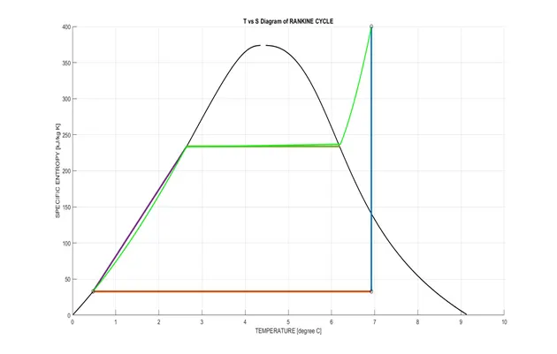
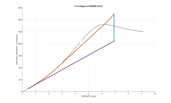
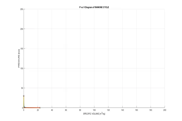
COMMAND WINDOW:
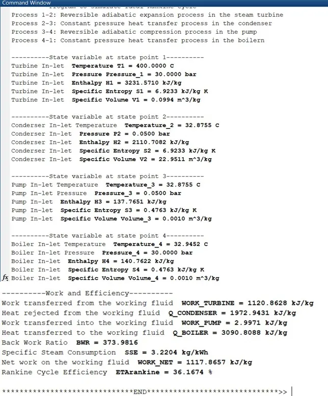
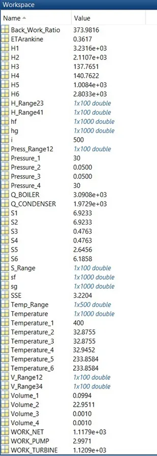
WORKSPACE: (for Pressure_1 = 30 bar, Pressure_2 = 0.05 bar, Temperature_1 = 400 C)
CONCLUSION:
Hence, we conclude that we successfully simulated the Rankine Cycle from the inputs from the user and plotted the graphs.