Week 4.1 - Genetic Algorithm

AIM:

Write a code in MATLAB to optimize the Stalagmite Function and find the Global Maxima of the function.

What is Stalagmite?

A stalagmite is a type of rock formation that rises from the floor of a cave due to the accumulation of material deposited on the floor from the ceiling drippings. Stalagmites are typically composed of calcium carbonate but may consist of lava, mud, peat, pitch, sand, sinter, and amberat (crystallized urine of packrats).

In MATLAB, the stalagmite function is a mathematical model that helps to generate local maxima and local minima.

Genetic Algorithm:

It is a search that is inspired by Charles Darwin’s theory of natural evolution. This algorithm reflects the process of natural selection where the fittest individuals are selected for reproduction in order to produce offspring of the next generation.

It’s a technique for solving both constrained and unconstrained optimization problems that are based on natural selection, the process that drives biological evolution. The Genetic Algorithm constantly modifies the population size of individual solutions.

Phases in Genetic Algorithm:

1. Initialization of Population (Coding):

The code generates its random population of defined size and from that population, the code evaluates the fitness of the members of the population, according to which it forms a new population which is based on the number of iterations performed.

• Fitness function:

A function which we have to optimize and its optimization is done with the help of the number of generations that have been formed by the code in accordance with the fitness value of each member-generated. These fitness values are used for the reproduction of children.

2. Selection:

The idea of the selection phase is to select the fittest individuals and let them pass their genes to the next generation.

The main goal of this phase is to find the region where the chances of getting the best solution are more. Inspiration for this is from the survival of the fittest.

There should be a balance between the exploration and exploitation of search space. GA tries to move the genotype to higher fitness in the search space.

TOO STRONG FITNESS SELECTION BIAS CAN LEAD TO SUB-OPTIMAL SOLUTIONS.

3. Reproduction:

Generation of offspring happens in 2 ways – i.). Crossover ii.). Mutation

i.). Crossover:

It’s the most significant stage in the genetic algorithm.

During crossover, a random point is selected while mating a pair of parents to generate offspring.

There are 3 major types of Crossover :

1. Single-Point Crossover – A point of both parents’ chromosomes is picked randomly, and designated a ‘crossover point’.
2. Two-Point Crossover – Two crossover points are picked randomly from the parent chromosomes.
3. Uniform Crossover – In this, typically, each bit is chosen from either parent with equal probability. THE NEW OFFSPRING ARE ADDED TO THE POPULATION.

ii.). Mutation:

In a few new offspring formed, some of their genes can be subjected to a mutation with a low random probability. This indicates that some of the bits in the bit-chromosome can be flipped.

Mutation happens to take care of the diversity among the population and stop premature convergence.

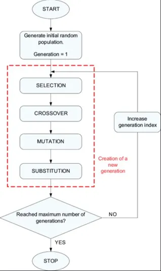
BASIC STRUCTURE OF GENETIC ALGORITHM:

GA() Initialize population find fitness of the population while (termination criteria is reached) parent selection crossover with probability pc mutation with probability pm decode & fitness calculation survivor selection find best return best

ADVANTAGES OF GENETIC ALGORITHM:

GAs have various advantages. These include:

• Doesn’t require any derivative information.
• Is faster & more efficient as compared to traditional methods.
• Has very good parallel capabilities.
• Optimizes both Continuous & Discrete functions and also multi-objective problems
• Provides a list of GODD SOLUTIONS, not just a single solution.
• Always gets an answer to the problem, which gets better over time.
• Useful when the search space is very large and there is a large number of parameters involved.

The genetic algorithm differs from a classical, derivative-based, optimization algorithm in mainly 2 ways –

CLASSICAL ALGORITHM	GENETIC ALGORITHM
Generates a single point at each iteration. The sequence of points approaches an optimal solution.	Generates a population of points at each iteration. The best point in the population approaches an optimal solution.
Selects the next point in the sequence by a deterministic computation.	Selects the next population by computation which uses random number generators.

How an algorithm performs :

• Begins by creating a random initial population.
• Scales the raw fitness scores to convert them into a more usable range of values. These scaled values are called expectation values.
• Then, selects the members, called Parents, based on their expectations.
• Along with the individual that has high fitness value, some of the individuals in the current population that have lower fitness are chosen as ELITE. These elite individuals are passed to the next population. Also, it produces Children by making random changes to a single parent – Mutation. Or by combining the vector entries of a pair of parents – Crossover.
• Then, it replaces the current population with the children to form the next generation.
• Scores each member of the current population by computing its fitness value. These values are called Raw Fitness Scores.
• The algorithm stops when one of the Stopping Criteria is met.

LIMITATIONS OF GENETIC ALGORITHM:

Like any other technique, GAs also have fewer limitations.

• GAs are not suitable for all problems, particularly simple problems with available derivative details.
• The fitness value is measured repeatedly, which can be computationally costly for certain problems.
• Since the solution is stochastic, there are no guarantees about its optimality or quality.
• If not implemented properly, the GA may not converge to the optimal solution.

APPLICATIONS OF GENETIC ALGORITHM:

GAs are primarily used in optimization problems of various kinds, but they are frequently used in other applications or areas as well. Such as –

• Economics – GAs are also used to characterize various economic models like Cobweb Model, Game Theory Equilibrium, Asset Pricing, etc.
• Neural Networks – They’re also used to train Neural Networks, particularly the Recurrent Neural Network.
• Image Processing – It’s also used for various Digital Image Processing tasks as well, like the Dense Pixel Matching.
• Parallelization – GAs have very good Parallel Capabilities, and prove to be very effective means in solving certain problems. They also provide a good area for research.
• Scheduling applications – GAs are used to tackle a variety of scheduling issues, most notably the timetabling problems.
• Machine Learning – Genetic-based machine learning is a niche area in machine learning.
• Vehicle Routing Problems – With multiple soft time windows, multiple depots, and a heterogeneous fleet.
• DNA Analysis – Using spectrometric data from the sample, GAs are used to determine the composition of DNA.
• Traveling Salesman Problem and its Application – Using novel crossover and packaging methods, GAs are used to solve the TSP, a well-known combinational challenge.
• Multi-Modal Optimization – GAs are obviously very approaching for multi-modal optimization in which we have to find multiple optimum solutions.

SYNTAX OF GA:

f_min = ga (@function, nvars, A, B, Aeq, Beq, LB, UB, nonlcon, intcon, options)

where

1. f_min = Local Minima Point
2. @Function = Function to be called
3. Nvars = Number of Variables Used
4. A, B = Used to Indicate Any Kind of Inequalities that Existed in Function.
5. Aeq, Beq = Used to Indicate Any Kind of Equalities that Existed in Function.
6. LB = Lower Bound Limit
7. UB = Upper Bound Limit
8. nonlcon = Used for Non-Linear Constraints
9. intcon = To Get Solution in Integer.
10. Options = Used to Perform Additional Operations Like Increasing Population Size. This is Done USING OPTIMOOPTIONS.

PROCEDURE:

• Separate definition of Stalagmite function, which is later called into the main GA program.
• Inputs (x, y) are defined using linspace command.
• These input vectors are transformed into an array [xx, yy] such that they can be used to evaluate the functions of 2 variables and plot a mesh.
• By calling the function which we created, Stalagmite Function, values in a different matrix can be put as input into the function. By this, we can get the different values of the function at various values of x & y.
• To calculate the Maxima, we use an in-built MATLAB function called “ga”.
• The total time required by “ga” to run is defined by using number_of_Cases. And by using For-Loop, each iteration is ran and the value is stored in an array.
• “ga” generally gives minimum value, but here we need maxima, so we inverse the stalagmite function using the ‘-‘ sign.
• Total study time is calculated using TIC & TOC
• The results are then plotted using the “surf” and “plot” command.

STALAGITE FUNCTION:

f(x, y) = f1x . f1y . f2x . f2y

f1x = (sin (5.1πx + 0.5))⁶

f1y = (sin (5.1πy + 0.5))⁶

f2x = exp [-4 ln(2) . `(x-0⋅667)^2/(0⋅64)]

f2y = exp [-4 ln(2) . `(y-0⋅667)^2/(0⋅64) ]

function[f] = stalagmite_func(input);
x = input (1);
y = input (2);
f1_x = (sin (5.1 * pi.*x + 0.5)).^6;
f1_y = (sin (5.1 * pi.*y + 0.5)).^6;
f2_x = exp (-4 * log(2).* ((x - 0.0667).^2 / 0.64));
f2_y = exp (-4 * log(2).*((y - 0.0667).^2 / 0.64));
f = -[f1_x.*f1_y.*f2_x.*f2_y];
end

PROGRAM:

Code for finding Global Maxima:

%% Code for finding Global Maxima

close all
%clear all
clc

%% Defining the search space
x = linspace (0, 0.6, 150);
y = linspace (0, 0.6, 150);

%% Creating 2-D array
[xx, yy] = meshgrid (x, y);

%% Calculating the Fitting function
for i = 1 : length (xx)
    for j = 1 : length (yy)
        input (1) = xx (i, j);
        input (2) = yy (i, j);
        
        f(i,j)= stalagmite_func (input);     % Values of function given
                                             % in search space.
          
    end
end


%% Converting the Fitting function to change the Graph upwards
F = -f;

%% Plotting the STALAGMITE function
surface (xx, yy, F);        % Generating the surface
shading interp              % To remove the lines generated by mesh-grid.
hold on;

%% Performing the GENETIC ALGORITHM
[output, fval] = ga(@stalagmite_func, 2, [], [], [], [], [0, 0], [0.6, 0.6]);

%% Plotting the GLOBAL MAXIMA
X_MAX = output (:, 1);
Y_MAX = output (:, 2);
F_MAX = -fval;

plot3 (X_MAX, Y_MAX, F_MAX, 'marker', 'o', 'markersize', 5, 'markerfacecolor', 'r');

xlabel ('X-Value');
ylabel ('Y-Value');
title ('GLOBAL MAXIMA');
legend ('STALAGMITE', 'GLOBAL MAXIMA');
grid on

OUTPUT:

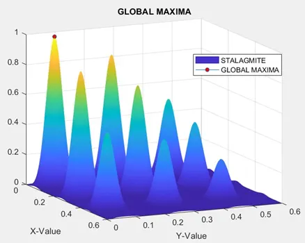
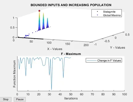
Iteration – 1:

The behavior of the algorithm is by not defining the limits. Since the bounds are not defined, GA doesn’t run within a particular search space.

Code for Statistical Behaviour:

%% Optimization :
%        It's basically the area of study that deals with how to Minimize
%        or Maximize a function that depends on multiple input parameters.

%% Genetic algorithm, Ga : 
%        It's a search-based optimization technique based on the principles
%        of Genetics and Neural Selection. It's frequently used to find the
%        optimal or near-optimal solutions to difficult problems which
%        otherwise would take a lifetime to solve.

%% Stalagmite function : 
%        It's a mathematical model that actually helps to generate local
%        maxima and local minima. 

close all
clear all
clc

%% Generating 1-D Array
x = linspace(0, 0.6, 150);
y = linspace(0, 0.6, 150);
number_of_Cases = 50;           % Number of iterations for which the 
                                % function will evaluate the fitness.

%% Generating 2-D Array
[xx, yy] = meshgrid (x, y);
 
%% Calculating Fitting Function
for i = 1 : length (xx)
    for j = 1 : length (yy)
        input (1) = xx (i, j);
        input (2) = yy (i, j);
        f (i, j) = stalagmite_func (input);     % Values of function given
                                                % in search space.
    end
end

F = -f;

%% Study 3 - Increasing iterations
options = optimoptions ('ga');
%options = optimoptions ('ga', 'PlotFcn',{@gaplotbestf,@gaplotstopping},'PopulationSize', 600);
                               % GAPLOTBESTF - Plots the best and mean 
                               %               score of population at 
                               %               every generation.
                               
                               % GAPLOTSTOPPING - Plots the percentage of 
                               %                  stopping criteria 
                               %                  satisfied.
                               
options = optimoptions (options, 'PopulationSize', 600);

%% Performing the Genetic Algorithm
tic       % Calculating the study time.
for L = 1 : number_of_Cases
    % Calculating the optimized value of the function at each iteration
    [inputs, fopt(L)] = ga (@stalagmite_func, 2, [], [], [], [], [0; 0], [1; 1], [], [], options);      
    xopt (L) = inputs (1);                   
    yopt (L) = inputs (2);                  % 
end

Fopt = -fopt;
study1_time = toc;      % Displaying the time taken to evaluate.

fprintf ('\n Study 1 : Unbounded Statistical Behaviour')
fprintf ('\n The Time taken for the study 1 is : %f', study1_time)
fprintf ('\n The Co-ordinates of x and y for the Global Maxima of the Function are : %f, %f', inputs (1), inputs (2))
fprintf ('\n The Global Maxima of the Function is : %f', -(mean(fopt)))
%% Plotting Global Maxima And function values
figure (1)
subplot (2, 1, 1);
hold on
surface (x, y, F);          % Generating the surface

shading interp              % To remove the lines generated by mesh-grid.

plot3 (xopt, yopt, Fopt, 'o', 'markersize', 5, 'markerfacecolor', 'r');
title ('Bounded Inputs And Increasing Population');
xlabel ('X-values');
ylabel ('Y-values');
legend ('Stalagmite','Global Maxima');
grid on
subplot(2,1,2)
hold on
plot (Fopt)
title ('F Maximum');
xlabel ('Iterations');
ylabel ('Function Maximum');
legend ('Change in F values');

OUTPUT:

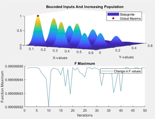
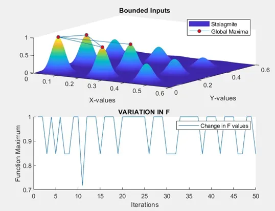
2. Iteration – 2: (Statistical behavior with Bounded Input)

Here, the lower and upper bounds are defined so as to know the boundaries within which the global maxima lie. In other words, we’re defining a definite space within which the global maxima is to be found.

Code:

close all
clear all
clc

%% Generating 1-D Array
x = linspace (0,0.6,150);
y = linspace(0,0.6,150);
number_of_Cases = 50;           % Number of iterations for which the 
                                % function will evaluate the fitness.

%% Generating 2-D Array
[xx, yy] = meshgrid (x, y);
 
%% Calculating the Fitting Function
  for i = 1 : length (xx)
      for j = 1 : length (yy)
          input (1) = xx (i, j);
          input (2) = yy (i, j);
          f (i, j)= stalagmite_func (input);     % Values of function given
                                                 % in search space.
      end
  end 
  F = -f;

%% Performing the Genetic Algorithm
tic        % Calculating the study time.
for L = 1 : number_of_Cases
    % Calculating the optimized value of the function at each iteration
    [inputs, fopt(L)] = ga(@stalagmite_func, 2, [], [], [], [], [0; 0], [0.6; 0.6]);
    xopt (L) = inputs (1);
    yopt (L) = inputs (2);
end

Fopt = -fopt;
study2_time = toc;      % Displaying the time taken to evaluate.

fprintf ('\n Study 2 : Bounded Statistical Behvaiour')
fprintf ('\n The Time taken for the study 2 is : %f', study2_time)
fprintf ('\n The Co-ordinates of x and y for the Global Maxima of the Function are : %f, %f', inputs (1), inputs (2))
fprintf ('\n The Global Maxima of the Function is : %f', -(mean(fopt)))
%% Plotting Global Maxima And function values
figure (1)
subplot (2, 1, 1);
hold on
surface (x, y, F);          % Generating the surface

shading interp              % To remove the lines generated by mesh-grid.

plot3 (xopt, yopt, Fopt, '-o', 'markersize', 5, 'markerfacecolor', 'r');
title ('Bounded Inputs');
xlabel ('X-values');
ylabel ('Y-values');
legend ('Stalagmite','Global Maxima');

subplot(2,1,2);
hold on
plot (Fopt);
title ('VARIATION IN F ');
xlabel ('Iterations');
ylabel ('Function Maximum');
legend ('Change in F values');

OUTPUT:

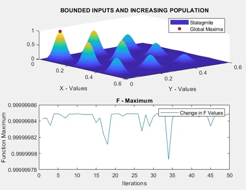
3. Iteration – 3: (Statistical Behaviour with Bounded Inputs and Increased Population)

In this iteration, the population size is increased so as to converge the Global Maxima.

Code:

% Code for Statistical behavior with bounded inputs and increased
% population

close all
clc

%% Generating 1 - D Array
x = linspace (0, 0.6, 150);
y = linspace (0, 0.6, 150);
number_of_Cases = 50;       % Number of iterations for which the 
                            % function will evaluate the fitness.

%% Generating 2 - D Array
[xx, yy] = meshgrid (x, y);

%% Calculation of Fitting Function
for i = 1 : length (xx)
    for j = 1 : length (yy)
        input (1) = xx (i, j);
        input (2) = yy (i, j);
        
        f (i, j) = stalagmite_func (input);     % Values of function given
                                                % in search space.
    end
end

F = -f;

%% Study - 3, Increasing Iterations
% Increasing the size of the population using OPTIMOPTIONS.
%options = optimoptions ('ga');  %, 'PlotFcn',{@gaplotbestf,@gaplotstopping},'PopulationSize', 600);          
options = optimoptions ('ga', 'PlotFcn',{@gaplotbestf,@gaplotstopping},'PopulationSize', 600);          
                               % GAPLOTBESTF - Plots the best and mean 
                               %               score of population at 
                               %               every generation.
                               
                               % GAPLOTSTOPPING - Plots the percentage of 
                               %                  stopping criteria 
                               %                  satisfied.
options = optimoptions (options, 'PopulationSize', 600);

%% Performing the Genetic Algorithm
tic         % Displaying the Study Time
for L = 1 : number_of_Cases
    % Calculating the optimized value of the function at each iteration
    [inputs, fopt(L)] = ga (@stalagmite_func, 2, [], [], [], [], [0; 0], [1; 1], [], [], options);
    xopt (L) = inputs (1);
    yopt (L) = inputs (2);
end

Fopt = -fopt;
study3_time = toc;          % Displaying the Time Taken to Evaluate

fprintf ('\n Study 3 : Bounded Statistical Behaviour with Increased Population Size')
fprintf ('\n The Time taken for the study 3 is : %f', study3_time)
fprintf ('\n The Co-ordinates of x and y for the Global Maxima of the Function are : %f, %f', inputs (1), inputs (2))
fprintf ('\n The Global Maxima of the Function is : %f', -(mean(fopt)))

%% Plotting the Global Maxima and the Function Values
figure (1)
subplot (2, 1, 1);
hold on
surface (x, y, F);          % Generating the surface

shading interp

plot3 (xopt, yopt, Fopt, 'o', 'markersize', 5, 'markerfacecolor', 'r');
title ('BOUNDED INPUTS AND INCREASING POPULATION');
xlabel ('X - Values');
ylabel ('Y - Values');
legend ('Stalagmite', 'Global Maxima');

subplot (2, 1, 2);
plot (Fopt);
title ('F - Maximum');
xlabel ('Iterations');
ylabel ('Function Maximum');
legend ('Change in F Values');

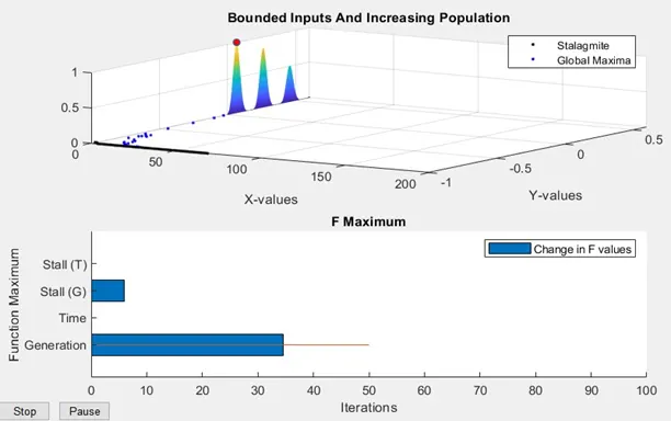
OUTPUT:

CONCLUSION:

It can be inferred that GA produces more reliable results when the inputs are bounded and the number of iterations and population size is increased.

It can also be deduced that even though we specify a certain search space for GA, GA does not run inside it. We can only get interfered results where the inputs are bounded.