Solving second order ODEs

AIM:

To solve the 2^nd Order Ordinary Differential Equation (ODE) and use animate the motion of the Pendulum using MATLAB.

INTRODUCTION:

A simple pendulum is defined to have a point mass, also known as the pendulum bob, which is suspended from a string of length L with negligible mass. Here, the only forces acting on the bob are the force of gravity (i.e., the weight of the bob) and tension from the string. The mass of the string is assumed to be negligible as compared to the mass of the bob.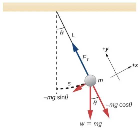

Length of Wire/String = L, Mass of bob = M, Theta (θ) = Angle corresponding to the vertical.

In the figure, tangential and radial components of gravitational forces are acting upon the bob. The radial force is balanced by the force exerted by the string. The tangential component of the gravitational force is responsible for producing the motion.

Ordinary Differential Equation:

It’s a differential equation containing one or more functions of one independent variable and the derivatives of those functions. The equation of an ODE is –

(d^2 θ)/(dt^2 )+B/M dθ/dt+g/L sin⁡θ=0 … Eq. – 1

θ= θ1

=> dθ/dt= dθ1/dt= θ2 … Eq. – 2

Also,

(d^2 θ)/(dt^2 )= (d^2 θ1)/(dt^2 )= d/dt (dθ1/dt)= dθ2/dt … Eq. – 3

Now, substituting the values of Eq. 2 & Eq. 3 in Eq. 1,

=> dθ1/dt=dθ2, dθ2/dt = -B/M θ2-g/L sin⁡θ1

=> d/dt[θ1; θ2] = [θ2; -B/M θ2-g/L sin⁡θ1]

d/dt[θ1; θ2] is the solution vector.

MATLAB CODE:

clear all

close all

clc

B = 0.05; % Damping Coefficient

g = 9.81; % Gravity (g)

L = 1; % Length of the Spring (in m)

M = 0.1; % Mass of the bob (in kg)

% Initial conditions

theta_0 = [0 ; 5]; % Angular displacement = 0

% Angular velocity = 5

% Time points

t_span = linspace (0, 25, 499); % Time for which pendulum oscillates

% Solving the ODE

[t, results] = ode45(@(t, theta) ode_func2(t, theta, B, g, L, M), t_span, theta_0);

% Plotting the graph

frame = 1;

for i = 1 : length (results (:, 1))

X1 = 0; % start position on x-axis

Y1 = 0; % start position on y-axis

X2 = L * sin (results (i, 1)); % end position on x-axis

Y2 = -L * cos (results (i, 1)); % end position on y-axis

subplot (3, 2, [1:4])

plot ([X1, X2], [Y1, Y2], 'linewidth', 2, 'color', 'b')

hold on

plot(X2, Y2, '-o', 'markers', 20, 'markerfacecolor', 'g')

axis ([-1.5, 1.5, -1.5, 0.5])

title ('Pendulum Animation')

hold off

subplot (3, 2, 5)

plot (t, results (:, 1))

hold on

plot (t(i), results (i, 1), 'o', 'markers', 5, 'markerfacecolor', 'r')

hold off

title ('Displacement')

subplot (3, 2, 6)

plot (t, results (:, 2))

hold on

plot (t(i), results (i, 2), 'o', 'markers', 5, 'markerfacecolor', 'r')

hold off

title ('Velocity')

pause (0.03)

MOVIE (frame) = getframe(gcf);

frame = frame + 1;

end

% Movie-making of the pendulum animation

movie(MOVIE)

videofile = VideoWriter ('Pendulum.avi', 'uncompressed AVI');

open (videofile)

writeVideo (videofile, MOVIE)

close (videofile)

FUNCTION CODE:

function [dtheta_dt] = ODE_function(t, theta, B, g, L, M)

theta1 = theta(1)

theta2 = theta(2)

dtheta1_dt = theta2;

dtheta2_dt = -(B/M) * theta2 - (g/L) * sin (theta1);

dtheta_dt = [dtheta1_dt; dtheta2_dt];

end

CODE EXPLAINATION:

First, by using the commands CLEAR ALL, CLOSE ALL & CLC, data from the workspace is cleared, previous/current figures are closed or deleted and lastly, all the I/P and O/P are cleared from the Command Window, respectively.

Now, the input & variables are defined.

Damping Coefficient, B = 0.05

Gravity, g = 9.81

Length of the string/wire, L = 1

Mass of the bob, M = 0.1

Then, the angular velocity and the angular displacement along with the time span for which the pendulum will oscillate is also defined.

To solve the ODE, MATLAB function, Ode45 is used, which solves the ordinary or the partial differential equations using the numerical method. Ode45 takes 3 inputs, function to be integrated, time-span, and the initial conditions. And the result is calculated wrt time, t. [t, results].

And to solve the ODE, an ODE function is declared which accepts the values of t, theta, B, g, L, M, t_span, and theta_0.

So, the function called ODE_function is declared which accepts the values of t, theta, B, g, L, M. Then the 2^nd order ODE is split into 2-parts, dtheta_1 & dtheta_2. dtheta_1 & dtheta_2 are made into an array of single variable dtheta which is a column matrix.

Then position & swinging area of the pendulum is declared.

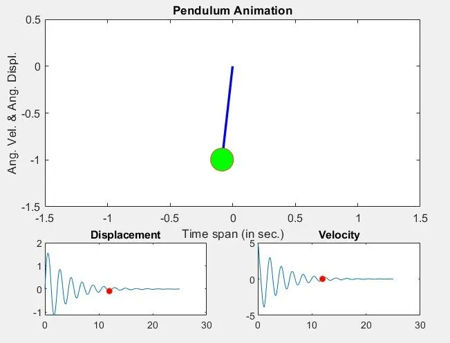
When the result is calculated, then the graph is plotted Angular Velocity and Angular Displacement vs Time.

An animation of oscillation of the pendulum is created and is captured frame-by-frame using the command getframe(gcf). An incremental loop counter, ct, is also used for multiple generations of frames.

Then, a movie file is generated and stored in format .avi.

ERRORS OCCURRED:

No major errors are encountered/faced except for missing operators and unwanted use of parenthesis.

OUTPUT:

Graph

https://youtu.be/Wj2gEvUys4s