Design of an Electric Vehicle

Design of an Electric vehicle

Introduction

Electric vehicles (EVs) are automobiles powered by electric motors, relying on rechargeable batteries or other energy storage devices for their energy source. Unlike traditional internal combustion engine vehicles that run on gasoline or diesel, EVs produce zero tailpipe emissions, making them a cleaner and more environmentally friendly transportation option. The popularity of electric vehicles has grown rapidly in recent years due to advancements in battery technology, increased environmental awareness, and government incentives promoting sustainable transportation. EVs come in various forms, including all-electric (battery electric vehicles - BEVs) and plug-in hybrid electric vehicles (PHEVs), offering consumers a range of options to reduce their carbon footprint and contribute to a more sustainable future

A new study related to Vehicle/Automobile engineering says that by coming 2025, there will be a major transformation in the automobile sector. Many automakers are working to change the vehicle technologies, the major area is to decrease the pollution and use electrification in the upcoming vehicles. The researchers and automakers are continuously working to reduce CO2 emissions.

New technology like high capacity lithium type battery will be a major energy source for the propulsion of electric vehicles.

At present, with the new technologies, some manufacturer has launched its products which are Tesla, Chevy Bolt EV and Nissan leaf,Tata punch, Tata Bolt, which are fully electric battery-based car.

The power and performance of electric vehicles is depending upon the two machines i.e. a brushless DC motor (BLDC) or an induction motor. The DC (direct current) is replaced by DC brushless motors and Induction motors. Also, the lead-acid battery is replaced by lithium-ion batteries for EVs. Because the future of both the components induction or brushless DC motors depends upon their demands and uses.

The most important components of electric vehicle areas:

1. Auxiliary Battery: In an electric drive vehicle, the auxiliary battery provides electricity to power vehicle accessories.
2. Traction Battery Pack: Traction battery pack is also known as Electric Vehicle Battery (EVB) which is used to store the electricity. Some examples of traction battery energy storage systems are as given:
   1. Lithium-Ion
   2. Nickel-Metal Hydride
   3. Lead-Acid
   4. Ultra-Capacitors
3. DC/DC Converter: Basically, DC/DC converter is an electronic device which is used to converts higher-voltage DC power from the traction battery pack to the lower-voltage DC power. The converted power is used to run the vehicle accessories. It is also used to recharge the auxiliary battery.
4. Electric Traction Motor: Another important component is electric traction motor and this device is used to provide motive power to the wheels.
5. Onboard charger: Takes the incoming AC electricity supplied via the charge port and converts it to DC power for charging the traction battery. It monitors battery characteristics such as voltage, current, temperature, and state of charge while charging the pack.
6. Power electronics controller: This unit manages the flow of electrical energy delivered by the traction battery, controlling the speed of the electric traction motor and the torque it produces.
7. Charge port: The charge port allows the vehicle to connect to an external power supply in order to charge the traction battery pack.
8. Thermal system (cooling): This system maintains a proper operating temperature range of the electric motor, power electronics, and other components.

MATLAB Modelling of Electric Car

Vehicle Technical Specification

• Vehicle Weight (Kg): 1147
• Number of wheels per axle: 2
• Total Length: 4.127 m or 4,127 mm
• Total Height: 1.487 m or 1,487 mm
• Total Width: 1.746 m or 1,746 mm

By Using MATLAB SIMULINK System Block for Electric Vehicle design and the whole design is as:

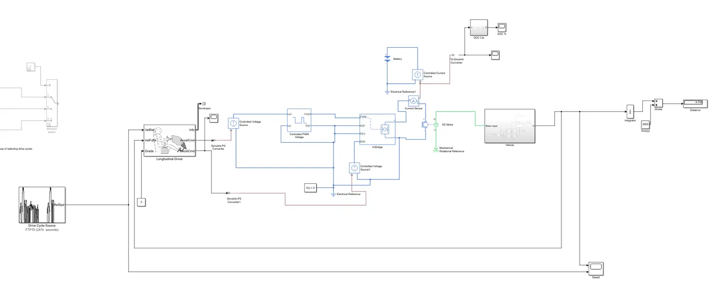
Important Simulink Block used in Electric Vehicle design are:

• Drive Cycle Source: 1
• Constant: 3
• Longitudinal Drive: 1
• Controlled Voltage Source: 2
• Controlled PWM Voltage: 1
• Solver Configuration: 1
• Electrical Reference: 2
• H-Bridge: 1
• DC Motor: 1
• Mechanical Rotational Reference: 1
• Current Sensor: 1
• Battery:1
• Controlled current source: 1
• PS-Simulink Converter: 4
• Vehicle Body: 1
• Tire: 4
• Simple Gear: 1
• Inertia: 1
• GoTo: 2
• PS Constant: 2
• Gain: 2
• Zero Order Hold: 1
• Rate Transition: 1
• Discrete Time Integrator: 1
• Sum: 1
• Integrator: 1
• Divide: 1
• Display: 1
• Scope: 4

MODELLING OF VEHICLE BODY SYSTEM:

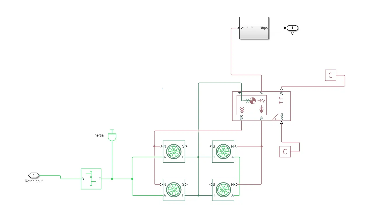
The Vehicle Body block represents a two-axle vehicle body in longitudinal motion. The vehicle can have the same or a different number of wheels on each axle.

The block consists of body mass, aerodynamic drag, road incline, and weight distribution between axles due to acceleration and road profile. In optionally we can include pitch and suspension dynamics.

The block has an option to include an externally-defined mass and externally-defined inertia. The mass, inertia, and centre of gravity of the vehicle body can vary over the course of simulation in response to system changes.

In a given block

1. NR: It is a physical signal output which is connected to the rear wheel axel. For this model, it is connected with a normal force of rear tire.
2. NF: It is a physical signal output which is connected to front-wheel axel and for this particular model it is connected with the normal force acting on a front-wheel tire.
3. Beta: Beta is basically a road incline angle. Here we can define a constant value for road angle inclination.
4. H: This port is a horizontal motion of the vehicle body. This connection will be connected with all four Hub of the wheel for finding the thrust generated by the tire.
5. V: This port is the vehicle longitudinal velocity.
6. W: It is a headwind speed. Basically, we will define a particular wind speed by adding constant block.

• For setup of vehicle body just double click on the vehicle body and enter as per requirement.
• Here I have done some changes in vehicle configuration, Basically, I changed the vehicle mass, length and frontal area.

• Detail input of Vehicle Body

Main Settings

1. Mass: 1147 Kg
2. Number of wheels per axle: 2

• The horizontal distance from CG to front axle: 1.854 m

2. The horizontal distance from CG to the rear axle: 2.2730 m
3. CG height above ground: 0.5 m
4. Externally-defined additional mass: OFF

• Gravitational acceleration: 9.81 m/s^2
• Negative normal force warning: OFF

Drag Settings

2. Frontal area: 2.21 m^2
3. Drag coefficient: 0.20

• Air density: 1.18 kg/m^3

Pitch Setting

1. Pitch dynamics: OFF

Variable Settings

1. Beginning Value of Velocity: 0 m/s

Other connected detail

• Wind Velocity: 2.22222 m/s
• Road Incline: 0

For calculating the velocity here, we have created a subsystem i.e LOG mph, this block basically consists of PS Simulink converter, Gain, Zero order Hold.

• Gain Block: 1.61 and it multiply input value with constant input.
• Zero-order Hold: 0.01, The Zero-Order Hold block holds its input for the sample period you specify.

TIRE MODELLING

The Tire (Magic Formula) block models a tire with longitudinal behaviour given by the Magic Formula, an empirical equation based on four fitting coefficients. The block can model tire dynamics under constant or variable pavement conditions.

The Tire (Magic Formula) block models the tire as a rigid wheel-tire combination in contact with the road and subject to slip. When torque is applied to the wheel axle, the tire pushes on the ground (while subject to contact friction) and transfers the resulting reaction as a force back on the wheel. This action pushes the wheel forward or backwards. If you include the optional tire compliance, the tire also flexibly deforms under load.

The figure shows the forces acting on the tire.

Where,

Fx = Longitudinal force exerted on the tire at the contact point

Fz = Vertical load on the tire

Ω = Wheel angular velocity

Vx = Wheel hub longitudinal velocity

In the particular block

• N: Normal force acting on the tire and connected with NR of the vehicle body.
• S: Slip between the tire and road and connected with Goto block
• H: Hub and it is used to find the thrust created by the tire and it is connected with H input of vehicle body also including all four Hub of the wheel.
• A: Axel and rear axle are connected with the (Simple Gear) final drive system and the front axle is connected with the left and right wheel.

In Tire block, we can change the parameter

Main Settings

• Parameterize by: Load-dependent Magic Formula coefficients, it is basically specifying the parameters that define the load-dependent.
• Tire nominal vertical load – This is basically a normal force on the tire (Fz0). So, for this particular model, the normal force I have taken is 4000 N.
• Magic formula C, D, E, BCD, H and V are default. Basically, It is a load-dependent Magic Formula Coefficient.

Geometry Setting

• Rolling radius: 0.32, it is Unloaded tire-wheel radius, rw

Dynamic Settings

• Inertia: Specify inertia and initial velocity which depends upon stiff, dampened spring and deforms under load.
• Tire inertia: 0.5 kg*m^2 and it is Rotational inertia Iw of the wheel-tire assembly.
• Initial velocity: 0 rpm and it is an Initial angular velocity, Ω(0), of the tire.

Rolling Resistance Setting

• Rolling resistance: On, Basically, it includes the rolling resistance.
• Resistance model: By using Constant Coefficient we are Neglect rolling resistance.
• Constant coefficient: 0.015 the value should be greater than 0 and it is a coefficient that sets the proportionality between the normal force and the rolling resistance force.
• Velocity threshold: 1e-3 m/s basically this input is a velocity at which the full rolling resistance force is transmitted to the rolling hub.

Advance setting

• Velocity threshold: 0.1 m/s as I keep this value as default and this value should be positive because it is wheel hub velocity Vth below which the slip calculation is modified to avoid singular evolution at zero velocity.

INERTIA

This block generally represents the mechanical rotational element.

Where,

T = Inertia torque

J = Inertia

Ω = Angular velocity

T = Time

So here the inertia value is 0.01 kg*m^2 and this block is connected with rear axle and (Simple Gear) final drive ratio to find the inertia because axel and gear are a mechanical rotating device.

SIMPLE GEAR

Simple Gear is a Final drive ratio which is a gearbox that constrains the connected driveline axes of the base gear and the follower gear.

B: The output B, base gear is connected with the input of DC motor R. It is a Rotational mechanical conserving port.

F: The output of F, follower gear is connected with the rear axle. It is also a Rotational mechanical conserving port.

In Simple Gear Block we can also do some changes according to our need.

Main Setting

• Follower (F) to base (B) teeth ratio (NF/NB): 2, The value should be in Positive and it is a fixed ratio gFB of the follower gear to the base gear.
• Output shaft rotates: In the same direction as the input shaft, it is depending upon the direction of follower and base gear.

Meshing Losses

• Friction model: From drop-down, we can select Constant efficiency which calculates the Reduce torque transfer by a constant efficiency factor.
• Efficiency: 0.86, here we can change the efficiency depending upon our need, basically it is a Torque transfer efficiency between base gear shaft to the follower gear shaft.
• Follower power threshold: 0.001 W, it is an absolute value of the follower shaft power above which the full efficiency factor is in effect.

Configuration Battery and SOC

BATTERY

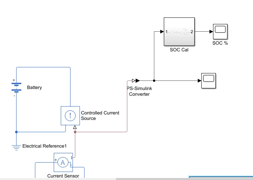
Here we will add a battery system to run the vehicle system and vehicle too. So for that added battery from Simulink library.

Here I used a simple battery model. For a particular battery, there is some changes input.

If we are selecting battery charge capacity as Finite from the drop-down menu then this basically describes the series resistor and a charge-dependent voltage source and for this, a particular equation is which is dependent upon the voltage as a function of charge.

Where,

• SOC (state-of-charge) is the ratio of current charge to-rated battery capacity.
• V0 is the voltage when the battery is fully charged at no load, as defined by the Nominal voltage, Vnom parameter.
• β is a constant that is calculated so that the battery voltage is V1 when the charge is AH1.

The connection of battery is as follow, the negative (-) terminal is connected with the ground and controlled current source physical port to the positive direction that indicates the flow.

The positive (+) terminal is also connected to the controlled current source of electrical conserving ports.

CONTROLLED CURRENT SOURCE

The Controlled Current Source block represents an ideal current source that is powerful enough to maintain the specified current through it regardless of the voltage across the source.

In this particular block, the two-port is connected with battery and one electrical conversing port is connected with PS-Simulink converter to the rate transition block and Scope block.

ELECTRICAL REFERENCE

The Electrical Reference block represents an electrical ground. For this model, this block is connected with battery negative (-) terminal.

PS-SIMULINK CONVERTER

The PS-Simulink Converter block converts a physical signal into a Simulink output signal. Use this block to connect outputs of a Physical Network diagram to Simulink scopes or other Simulink blocks.

For calculating the SOC (State of Charge) we have to create a subsystem which will consist of Rate transition, Gain, Discrete Time Integrator, Constant and Sum blocks.

RATE TRANSITION

It is used to transfers data from the output of a block operating at one rate to the input of a block operating at a different rate.

Input Signal: Input signal to transition to a new sample rate, specified as a scalar, vector, matrix, or N-D array.

Output Signal: Output signal is the input signal converted to the sample rate you specify.

A basic input for this block is as

GAIN BLOCK

The Gain block multiplies the input by a constant value (gain). The input and the gain can each be a scalar, vector, or matrix.

Here Gain value is the multiplication element and the input is 1/(50*3600), where 50is battery ampere and 3600 is second.

DISCRETE-TIME INTEGRATOR

The discrete-time integrator block is used for

• Define initial conditions on the block dialogue box or as input to the block
• Define an input gain (K) value
• Output the block state
• Define upper and lower limits on the integral
• Reset the state with an additional reset input

SUM BLOCK

The Sum block performs addition or subtraction on its inputs.

In this block, the negative terminal will be connected with discrete-time integrator and positive terminal with constant.

DETAIL ABOUT ELECTRICAL SYSTEM

DC MOTOR

The DC Motor block represents the electrical and torque characteristics of a DC motor using the following equivalent circuit model:

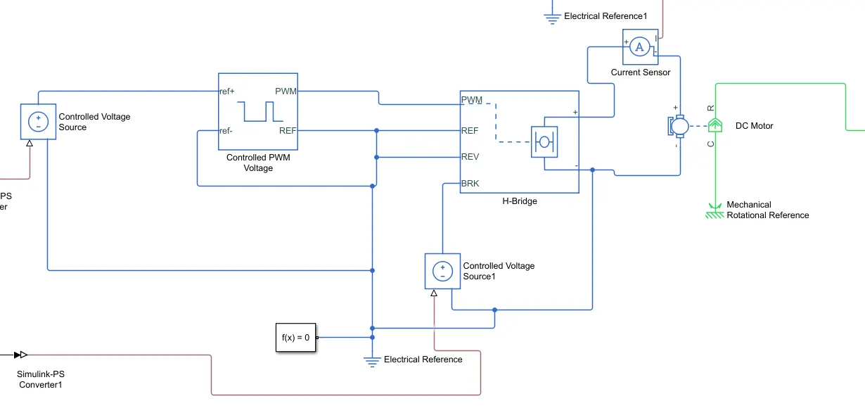
Here in this system, the positive terminal is connected with the current sensor negative terminal and negative terminal is connected with the negative terminal of H-Bridge.

R is DC motor rotor which connected with mechanical rotational port i.e. simple gear whereas C is DC motor case and it is connected with mechanical rotational reference.

A basic configuration of the DC motor is as follow:

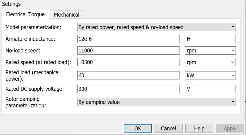
Here for the particular model, I configure in DC Motor and try to change a basic setting in electrical torque.

• No-load Speed: 11000 rpm, this is the speed of the motor when not driving a load.
• Rated speed (at load): 10500 rpm, this is the speed of the motor at rated mechanical power level.

Another Mechanical detail of DC motor is as follow

• Rotor Inertia: It’s a resistance of the rotor to change in motor motion.
• Rotor Damping: It should be zero because it is energy dissipated by the motor.
• Initial Rotor Speed: This is a starting speed of the motor that at what speed the motor will start.

H-BRIDGE

The H-Bridge block represents an H-bridge motor driver.

Simulation mode and Load Assumption Settings

• Power Supply: The power supply is default mode i.e. Internal.
• Simulation Mode: Here I selected Averaged mode and this mode has two Load current characteristics options:
• Regenerative Braking: Always enabled (suitable for linearization), this option can be used when the controller always sets the REV flag to ensure regenerative braking.
• Load Current Characteristics: Smoothed, it’s a default option and it assumes that the current is practically continuous due to load inductance.

Input Thresholds

• Enable threshold voltage: 1.5 V, this is the above value of PWM at which H-Bridge start.
• PWM signal amplitude: 5.0 V, this is the amplitude of the signal at the PWM input. Here I used it as the default mode.
• Reverse threshold voltage: 1.5 V, here I changed this value.
• Braking threshold voltage: 2.5 V

Bridge Parameters

• Output voltage amplitude: 320 V, this parameter will be active only when we select Internal for Power Supply mode and it’s an amplitude of the voltage across the H-Bridge.
• Total bridge on resistance: 0.1 ohms,
• The freewheeling diode on resistance: 0.05 ohm

Detail about connection

• PWM: Pulse-width modulated signal.
• REF: Reference, it is an electrical conversing port associated with the floating zero volts.
• REV: Reverse, it is an electrical conserving port associated with the voltage that controls when to reverse the polarity of the H-Bridge block output.
• BRK: BRK, it is an electrical conserving port associated with the voltage that controls when to short circuit the H-Bridge block output.

Here PWM output port is connected with PWM input port of controlled PWM voltage. The REF and REV port are connected with REF port of controlled PWM voltage port. The BRK port is connected with a controlled voltage source.

The positive (+) terminal is connected with the positive (+) port of current sensor and negative (-) port is connected with the negative (-) port of DC motor.

CONTROLLED PWM VOLTAGE

The Controlled PWM Voltage block represents a pulse-width modulated (PWM) voltage source. The input detail is as given below.

Detail about the connection

• ref+ — Positive terminal, this port is a positive electrical reference and connected with controlled voltage source positive terminal.
• ref- — Negative terminal, this port is a negative electrical reference and connected with the negative terminal of the controlled voltage source.
• PWM — Pulse-width modulated signal, this port is electrical reference port and connected with PWM port of H-Bridge.
• REF — Floating zero-volt reference, this port is connected with REF and REV of H-Bridge port.

CONTROLLED VOLTAGE SOURCE

The Controlled Voltage Source block represents an ideal voltage source that is powerful enough to maintain the specified voltage at its output regardless of the current flowing through the source.

The block has one physical signal input port and two electrical conserving ports associated with its electrical terminals.

SOLVER CONFIGURATION

Solver configuration is used to begin the simulation and it is needed to solve the Simulink model. Here it is connected with controlled PWM voltage and H-Bridge negative connection by combination with electrical reference i.e ground signal.

LONGITUDINAL DRIVER

The Longitudinal Driver block implements a longitudinal speed-tracking controller

The detail of inputs is as given

Detail about parameter

• Control Type: PI it is a Proportional-integral (PI) control with tracking windup and feed-forward gains.

• Reference and feedback unit: m/s

Detail about connection:

• VelRef: Reference vehicle velocity is connected with speed result block. Its unit is m/s.
• VelFdbk — Longitudinal vehicle velocity is connected with integrator block for continuous-time integration of VelFdbk signal.
• Grade — Road grade angle is connected with constant block so that we can use our specific value, here the value is 0 which I used.
• Info — Bus signal, Here I used this signal to terminate the signal block, basically it’s an output port.
• AccelCmd — Commanded vehicle acceleration is connected with controlled voltage source input signal by combination with PS-Simulink Convertor.
• DecelCmd — Commanded vehicle deceleration is connected with another controlled voltage source signal by combination with PS-Simulink converter and to check the output result I have connected with scope block.

DRIVE CYCLE SOURCE

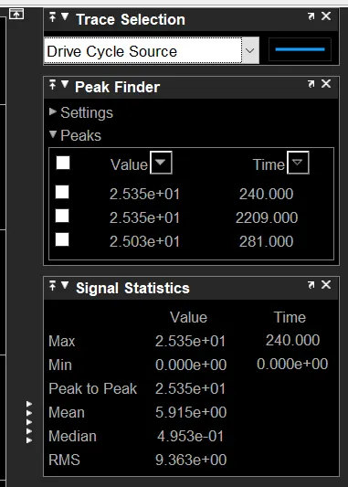
For this particular electric vehicle here I used FTP75 drive cycle. The plotted drive cycle is as given:

The connection drive cycle RefSpd is connected with the VelRef of Longitudinal driver and to the Scoop results which generate the vehicle reference speed.

DISTANCE CALCULATION

Here the main block is an integrator, Divide, time block and for the result we have to use display block that will display the distance.

Detail about connection:

Integrator

The output port of the vehicle body is connected with the integrator block.

Divide

The output of the integrator block is connected with divide where it will be divided by time to get the final output.

Time

The output of time block is connected with the divide block. Here time is taken as 3600 s.

RESULTS

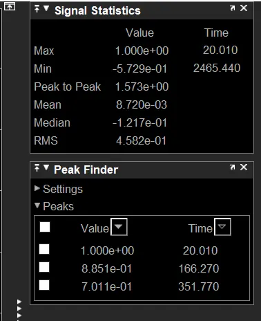
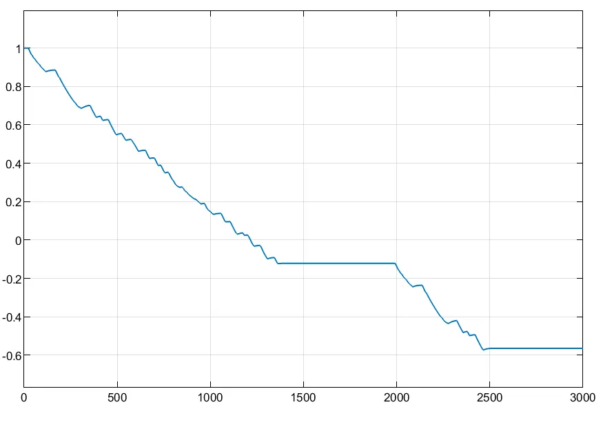
SOC %

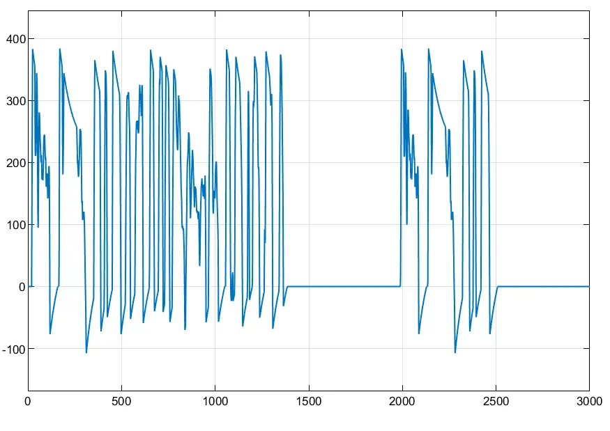
Current

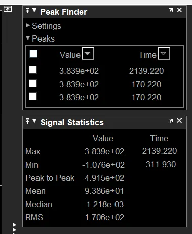
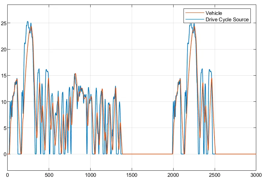
Speed

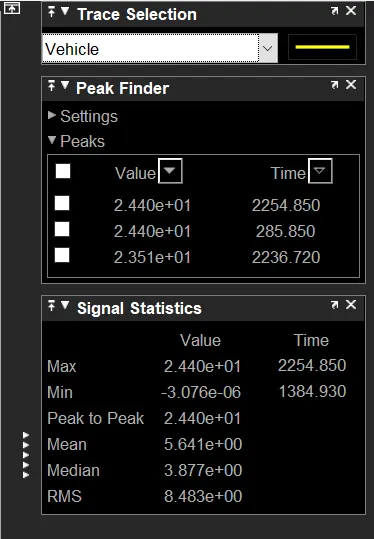
As we can see the difference time between the reverence speed Vs vehicle speed, this is basically starting of vehicle speed.

Conclusion:

The total distance travel by vehicle is 4.706m depending upon the FTP75 drive cycle and the total time for simulation was 3000sec.

The battery is having 300 V which is a nominal voltage and the battery ampere per hour rating is 60 by which we calculated the SOC (state of charge) of battery.

The DC motor is used to run the Rear axel of the vehicle and when the car is with no load condition then the motor operating RPM is 11000 and when the car is running at some load or we can say that some rated speed then the motor RPM is taken as 10500. The voltage supply to DC motor is 300 V.