Bird Strike Impact on Jet Engine Blades using LS-DYNA

Objective:

Simulate a dummy bird model strike on aero-engine blades. The material for the blades has been given. Elastic material has to be used for the bird and the casing. The bird approaches the blades at a high speed with the blades moving at a constant rotational velocity. The parts, nodes, elements and the keywords to be used should have a unique numbering system as stated in the challenge. One of the goals of this simulation is to organize the files in a folder and call them using *Include command. Mass scaling is to be used to decrease the runtime of the simulation and the results of mass-scaling are compared to the conventional approach.

Introduction:

Bird strikes have been a common occurrence in the history of aviation and have posed a threat to flight safety for years. They happen mostly during takeoffs or landing or during low-altitude flights. Usually, jet engine ingestion is the result of such a scenario due to the high rotational speed of the blades. The jet blades can be displaced into other blades resulting in cascading failure. The usual simulation is done using an advanced technique called Smoothed Particle Hydrodynamics (SPH). However, since the objective of this challenge is to learn the right techniques of LS-DYNA simulation and not simulate the actual scenario, SPH is not used.

The unit system used for this simulation is kg-mm-ms.

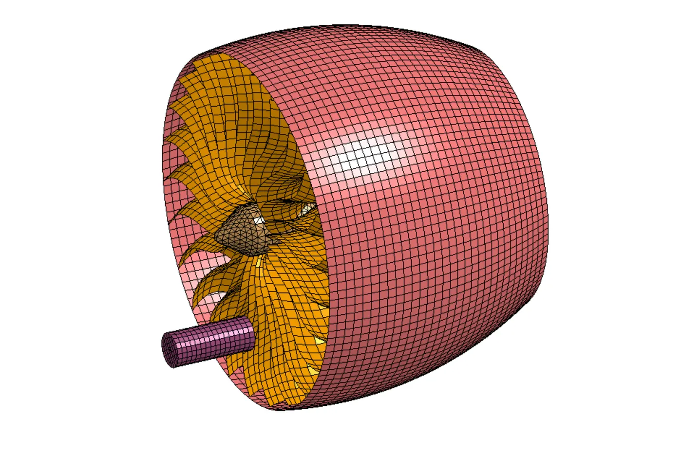
The study model for this simulation is:

Procedure:

Following are the steps followed for this simulation:

1) Seperating the component files

2) Creating and assigning materials to the components in a MAT file

3) Creating and assigning section to the components in a section file

4) Contact file to establish contact between bird and blades

5) Imparting velocity to the engine and the blade

6) Creating seperate files for control, database

7) Renumbering nodes and elements as given

8) Using the include command to call all the cards to a main file

Node_Set and Part_set were created for each component to use them while imparting boundary conditions to the model.

1) Creating individual components

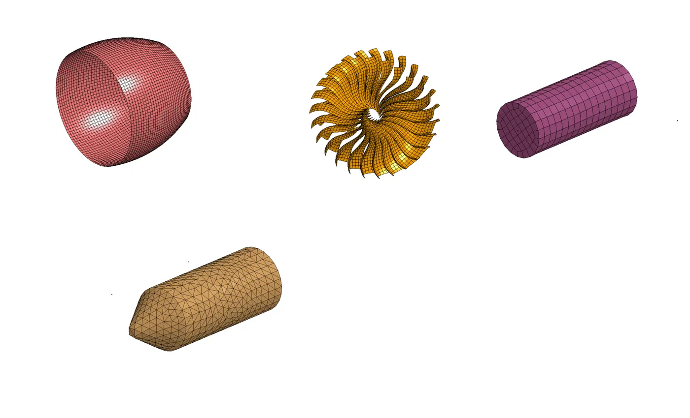
The model contains 4 components: Blades, hub, bird and Casing. These components have to be segregated into different component files. The method used to do this is to open the model containing all the components, delete 3 components by going to the assembly and saving the remaining component as a seperate .k file.

In this manner, the 4 individual components are created.

2) Material and section for the parts:

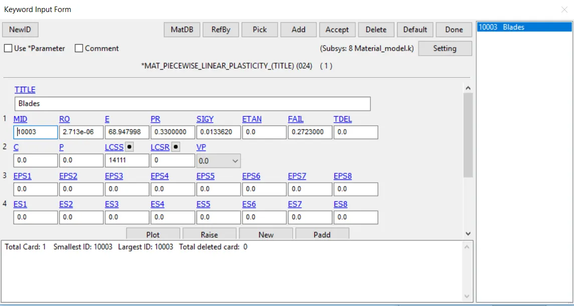
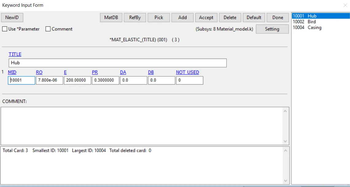
The material for blades has been given to us as an aluminum-titanium alloy. For the casing, and the hub, steel is used. The bird is usually modelled using SPH, but for this simulation, an elastic material similar to the human muscle is used.

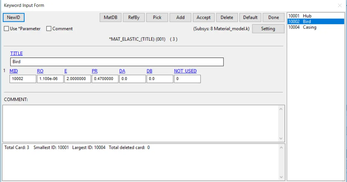
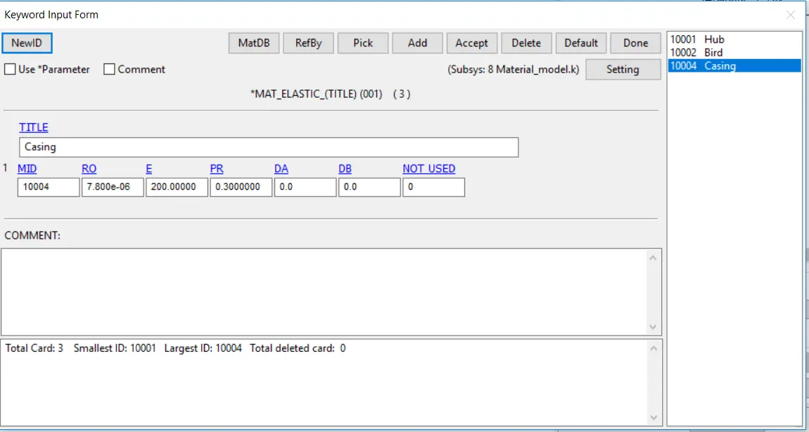
The section used for blades, Casing and bird is shell and element formulation used is 16. Solid elements are used for the hub with element section as 4.

3) Contact setup:

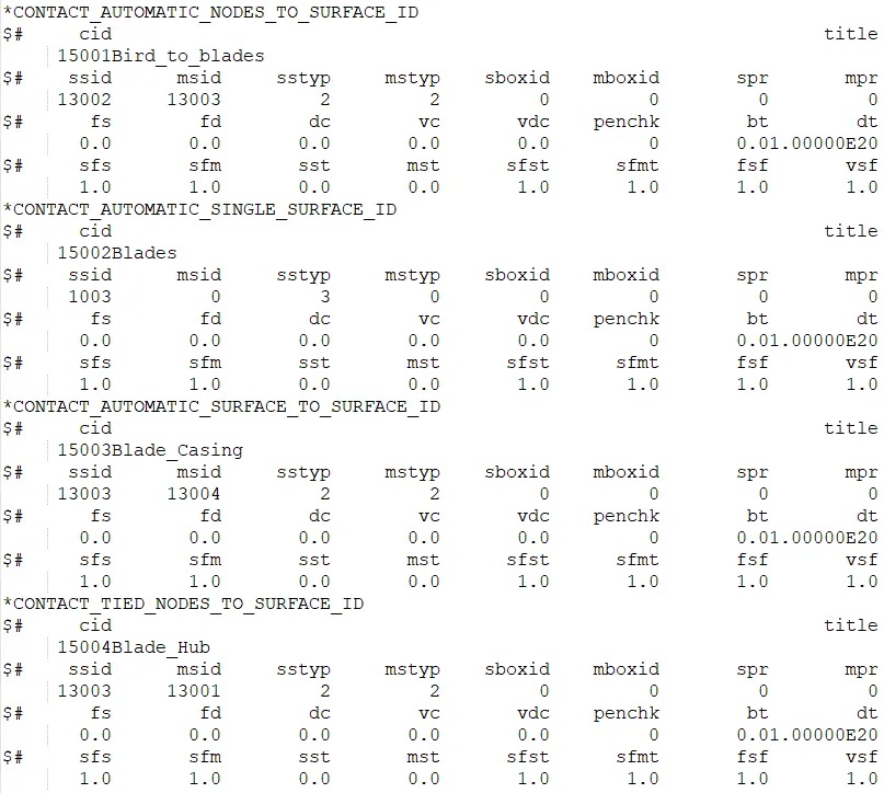
Conventionally, while using SPH, the contact card is used for defining contact between birds, blades and casing using *CONTACT_AUTOMATIC_NODES_TO_SURFACE. For this simulation as well, the *CONTACT_AUTOMATIC_SINGLE_SURFACE, *CONTACT_AUTOMATIC_NODES_TO_SURFACE and *CONTACT_AUTOMATIC_SURFACE_TO_SURFACE have been used. Basically, it is ensured that contact between all the components are considered in the simulation.

4) Boundary Conditions:

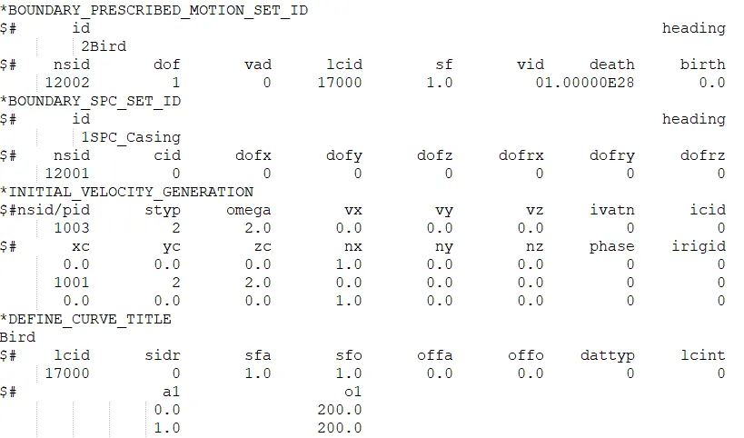
The conditions that are given here require the bird to go towards the aero engine. The velocity of the bird was 200 mm/ms. This was done by assigning the node-set created for the bird in the *Boundary_Prescribed_Motion card.

The blade and the hub were given a rotational velocity of 2. With higher rotational velocities, the simulation tended to be a bit unstable with the blades getting detached and flying outwards.

This was done using the *INITIAL_VELOCITY_GENERATION card.

5) *CONTROL:

The termination time for this simulation is given to be 10 ms. Apart from *CONTROL_TERMINATION, *CONTROL_HOURGLASS is used to interpret hourglass energy.

To track initial penetrations during contact, *Control_Contact has been used as well.

Likewise, to track hourglass energy, *Control_Energy has been used. *Control_Timestep card is also utilized in the simulation.

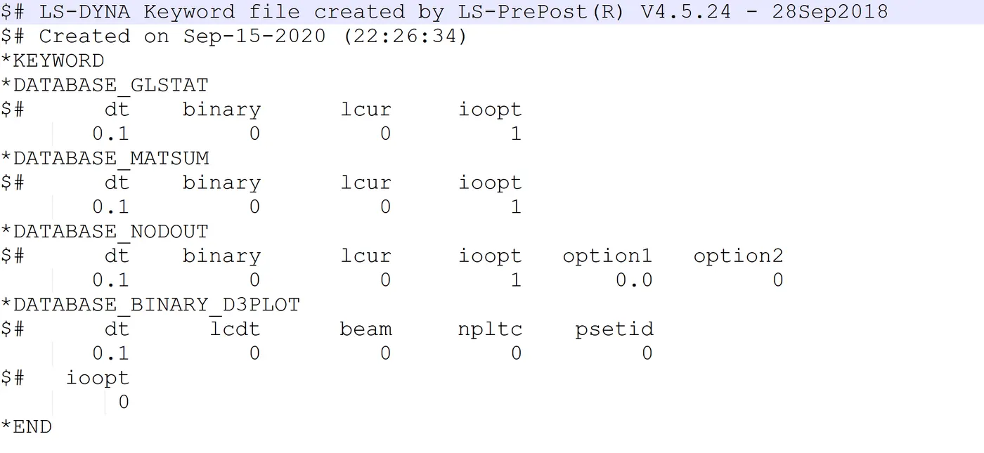
6) Database ASCII and database_extent_binary cards are used to get output files. GLSTAT, MATSUM, SLEOUT, RWFORCE are written

7) Renumbering:

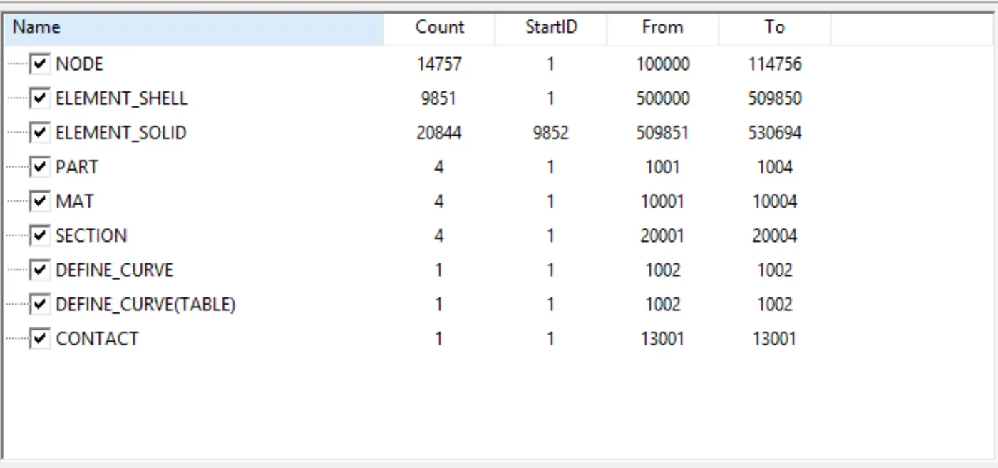
As mentioned before, the goal of this challenge is to organize the file according to the industry standards. A numbering system is used for denoting elements, nodes, parts, and other keywords. For example: 100000+ has been used for the nodes, 500000+ has been used for the elements and 1000+ has been used for the parts. All other keywords have also been numbered accordingly

	ID min	ID max	Casing	Blades	Hub	Bird
Node	100000	114421	106672-110768	100418-106671	110769-114756	100000-100417
Elements	500000	530694	505883-509850	500410-505882	509851-530694	500000-500409
Part	1001	1004	1004	1003	1001	1002
Section	20001	20004	20004	20003	20001	20002
Material	10001	10004	10004	10003	10001	10002
Contact	15001	15004	-	-	-	-
Control	-	-	-	-	-	-
Output	-	-	-	-	-	-

8) Include:

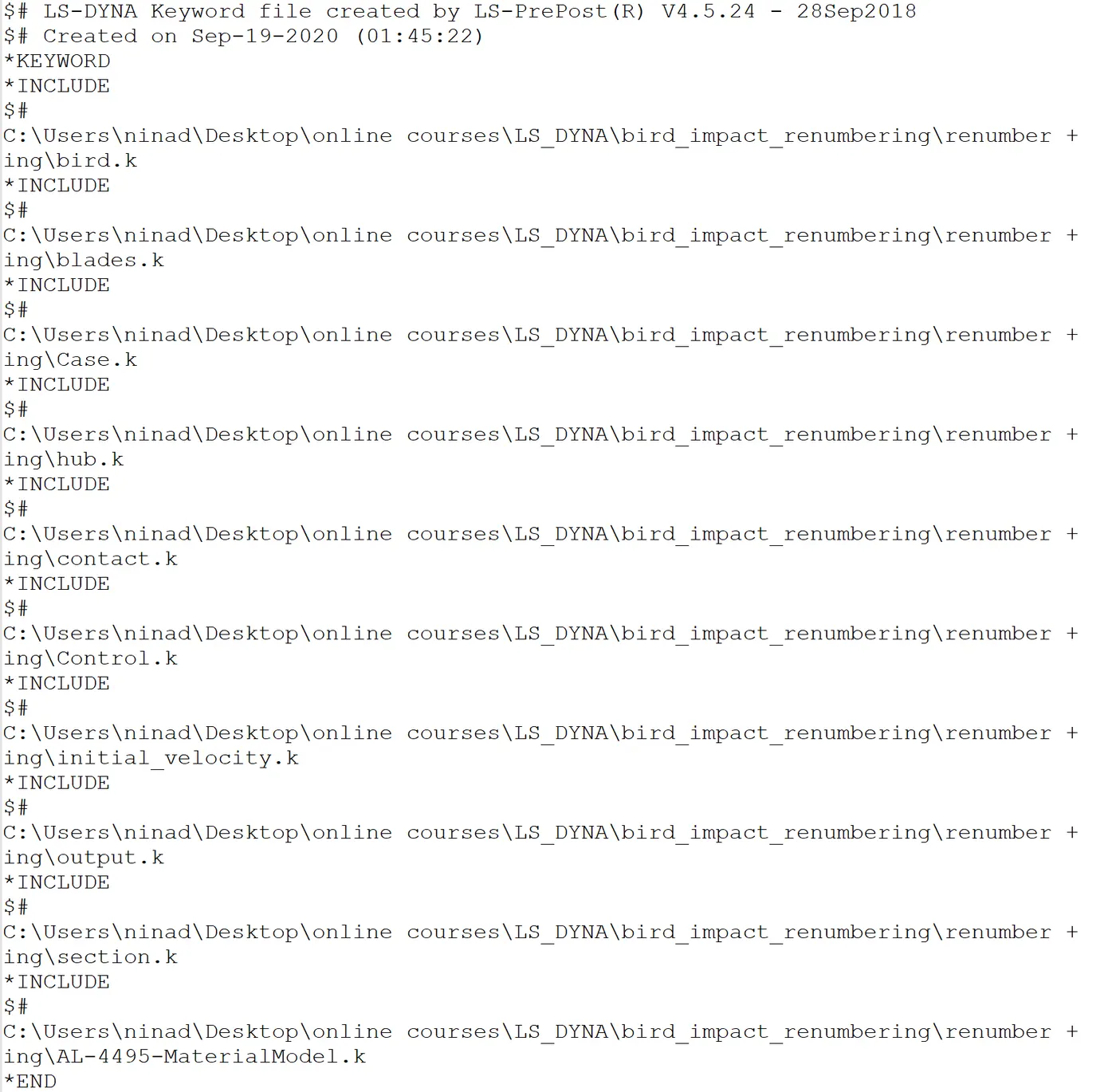
The above sections mention how separate files have been created for the purpose of this study. Individually, these files donot operate the way this study needs. They need to be merged and called in a file. For this case, all the files are called in a file called Main file.

*Include keyword has been used for this purpose and the files are called in the main file.

This method is the one actually used in the industry for conducting CAE simulations. As shown, all the keyword files are called and compiled in a main file for running the simulation.

The main file only has the following in it:

Debugging:

The process of running the simulation for this study was filled with errors and the initial error was not assigning section and material to the parts. Of course, this being a minor issue, the parts were assigned the section and material and the simulation was run again

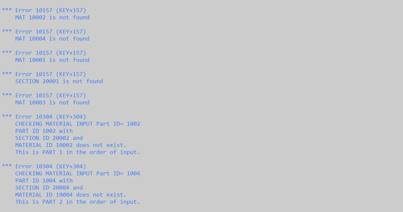
The second error was with d3plot interval. This, again, was a minor issue and was fixed.

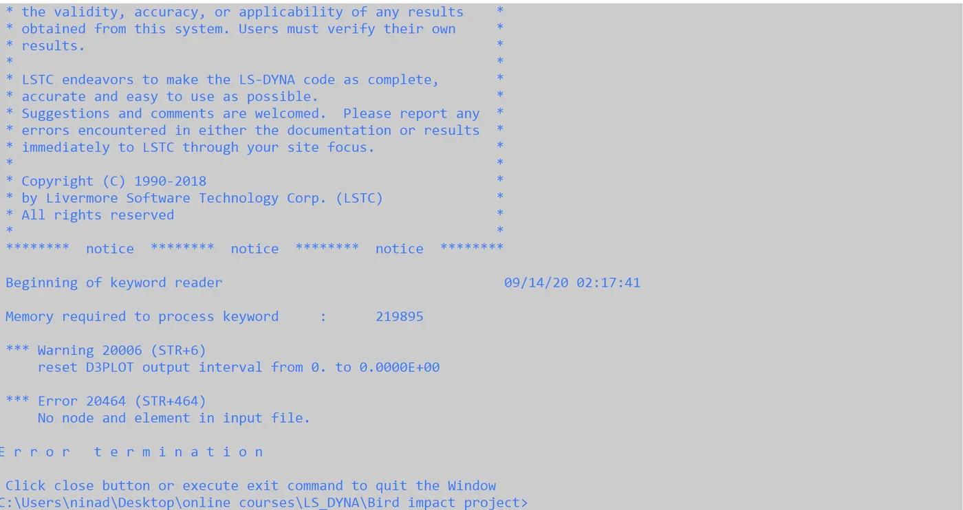
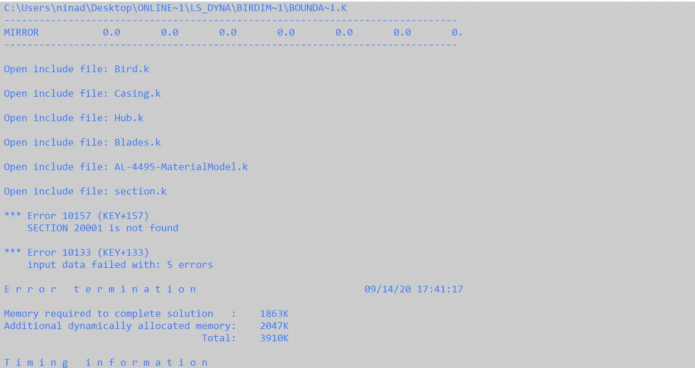
A faulty renumbering in the section card for the hub gave rise to the 3rd error as follows:

The final error was with mass scaling of the simulation. This was due to assigning a lower value of dt in the DT2MS box as compared to the original value. This simply resulted in deletion of all elements.

There were also certain instabilities with running the simulation for higher rotational speed of the blades. While doing so, the blades detached from the hub.

Results:

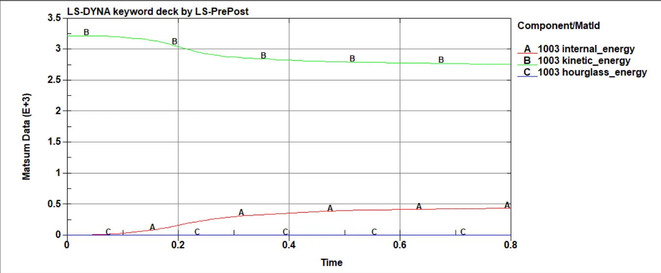
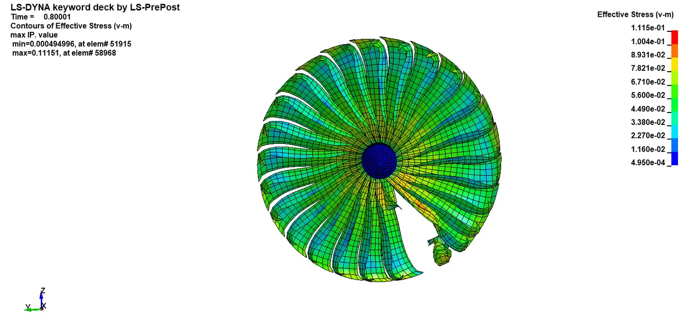
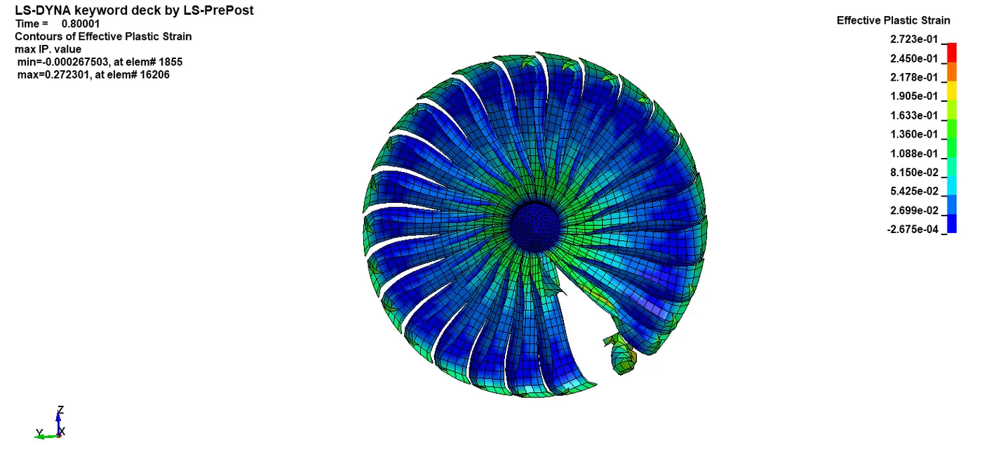
After compiling all the files, the simulation was run. The data extracted from the files is as follows:

Von-Mises Stress

Effective_Plastic_Strain

Mass- scaling:

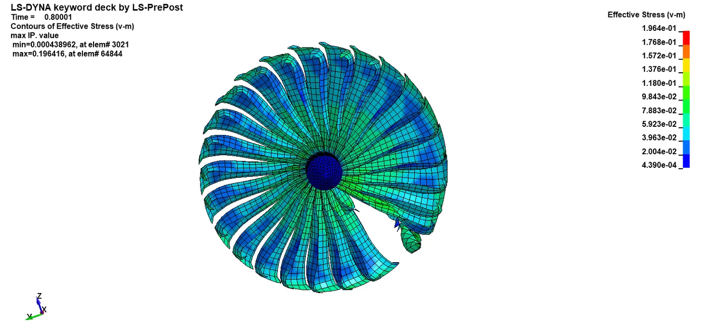
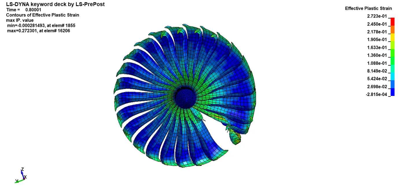
The simulation runtime for this case is around 50 mins. However, for complex scenarios like this, to reduce the similation time, mass-scaling is used. Hence, mass-scaling approach has been tried for this simulation with around 4% mass increase and the comparison of the results has been shown below:

	DT2MS	Physical Mass (kg)	Added Mass (kg)	Mass increase (%)	Simulation Time (sec)	Stress on Blades (GPa)	Strain on blades
Original	0	1.478	0	0	820	0.115	0.2723
Mass-Scaling	2.00E-04	1.478	0.048315	3.269	556	0.1946	0.2723

Mass scaling Von-Mises stress and strain:

VON-MISES

Effective Plastic Strain

Result:

This project helped me understand the procedure used to set up a complex model having dynamic characteristics and different components using include keyword. It also helped me understand the importance of mass scaling.