Week 2 Air standard Cycle

Aim: To write a code for plotting PV diagram of Otto cycle and determine the efficiency of the same.

Introduction:

An Otto cycle is an idealized thermodynamic cycle that describes the functioning of a typical spark ignition piston engine. It is the thermodynamic cycle most commonly found in automobile engines.

The Otto cycle is a description of what happens to a mass of gas as it is subjected to changes of pressure, temperature, volume, the addition of heat, and the removal of heat. The mass of gas that is subjected to those changes is called the system. The system, in this case, is defined to be the fluid (gas) within the cylinder. By describing the changes that take place within the system, it will also describe in the inverse, the system's effect on the environment. In the case of the Otto cycle, the effect will be to produce enough net work from the system so as to propel an automobile and its occupants in the environment.

Air standard cycle is a cycle in which air is used as a working substance or as a system.
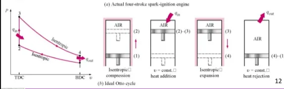
The Otto cycle is constructed from a pair of frictionless, adiabatic process and a pair of constant volume process.
The processes are described by the following:
Process 0–1 a mass of air is drawn into piston/cylinder arrangement at constant pressure.
Process 1–2 is an adiabatic (isentropic) compression of the charge as the piston moves from the bottom dead center (BDC) to top dead center (TDC).
Process 2–3 is a constant-volume heat transfer to the working gas from an external source while the piston is at the top dead center. This process is intended to represent the ignition of the fuel-air mixture and the subsequent rapid burning.
Process 3–4 is an adiabatic (isentropic) expansion (power stroke).
Process 4–1 completes the cycle by a constant-volume process in which heat is rejected from the air while the piston is at the bottom dead center.

The following assumptions are employed in the calculation. These are commonly known as the air standard assumptions:
1- The working fluid is air, which continuously circulates in a closed loop (cycle).
Air is considered an ideal gas.
2- All the processes in (ideal) power cycles are internally reversible.
3- The combustion process is modeled by a heat-addition process from an external
source.
4- The exhaust process is modeled by a heat-rejection process that restores the
working fluid (air) at its initial state.

Formulae governing the equations are as follows:
1) Isentropic process: `PV^(gamma) =`Constant
Isochoric process: `P/T` = Constant

2) Ideal gas equation: `(PV)/T =`Constan`

3) Compression Ratio: `C= (V_s+V_c)/(V_c)`

4) Change of volume inside the combustion chamber during expansion and compression is given by the following :
`V/V_c = 1+1/2(CR-1)[R+1 - cos(theta) - (R^2 - (sin^2(theta)))^0.5]`

5) Thermal Efficiency:
`eta = 1 - 1/(CR)^(gamma-1)`

where,

P = pressure(N/m^2)
CR = Compression Ratio
T = Temperature (K)
`gamma` = ratio of specfic heat
`V_s` = Swept volume
`V``V_c = Compression ratio`
R = Crankpin radius

Code procedure:
1) A starting crank angle and an ending crank angle are given as input along with parameters like bore diameter, stroke length, and length of the connecting rod.
2) Using a function, first, we get a range of angles between 0 and 180.
3) Using the formula for isentropic expansion and compression, the expansion volume and compression volume are obtained for each value of theta between 0 and 180.
4) Using the ideal gas and isentropic equation, the volume, pressure, and temperature are computed at each state point.
Note: Volume at 2nd and 3rd state points are the same given isochoric heat addition. The same is the case for 4th and 1st state points due to isochoric heat rejection.

Code:

import math
import matplotlib.pyplot as plt

#fucntion definition for extracting the v_expansion and v_compression
def engine_kinematics(bore,stroke,con_rod,cr,start_crank,end_crank):

	#geometric parameters
	a = stroke/2
	R = con_rod/a


	#clearance volume and swept volume calculations
	v_s = (math.pi/4)*pow(bore,2)*stroke
	v_c = v_s/(cr-1)
	v1 = v_c + v_s
	v2 = v_c
	#in here, we also calculate the theta angles, compression volume and compression pressure
	num_values = 50
	s = math.radians(start_crank)
	e = math.radians(end_crank)
	dtheta = (e-s)/(num_values-1)
	theta = []

	for i in range(0,num_values):
		t = s + i*dtheta
		theta.append(t)

	#now, we can use the theta values to calculate the volume as follows:
	V = []

	for dt in theta:
		term1 = 0.5*(cr-1)
		term2 = R+1-math.cos(dt)
		term3 = pow(pow(R,2)-pow(math.sin(dt),2),0.5)

		v = (1 + term1*(term2-(term3)))*v_c
		V.append(v)
	return(V)

# now, we need to define the values of p1,v1,p2,v2,p3,v3,p4,v4,t1,t2,t3,t4
#Following is the calculation procedure using isentropic process and isochoric process formulae
stroke = 0.1
bore = 0.1
con_rod = 0.15
cr = 10


p1 = 101325
t1 = 500
gamma = 1.4
# temperature at data point 3 (in K)
t3 = 2300

#geometric parameters
a = stroke/2
R = con_rod/a

#clearance volume and swept volume calculations
v_s = (math.pi/4)*pow(bore,2)*stroke
v_c = v_s/(cr-1)
v1 = v_c + v_s
v2 = v_c

#using p1v1^(gamma) = p2v2^gamma, p2 = p1v1^(gamma)/v2^(gamma)
rhs = p1*pow(v1,gamma)
p2 = (rhs)/pow(v2,gamma)
print(p2)
	
#using p1v1/t1 = p2v2/t2 = p3v3/t3 = p4v4/t4 = const, we calcuate the value of t2
const = p1*v1/t1
t2 = p2*v2/const


#now we can calculate state point 3 parameters:
v3 = v2

#using p1v1/t1 = p2v2/t2 = p3v3/t3 = p4v4/t4 = const, we calcuate the value of t2
p3 = const*t3/v3
print(p3)
#to calculate the parameters at state point 4, we know that v4 = v1
v4 = v1

#using pv^gamma relation, we can calculate p4
p4 = p3*pow(v3,gamma)/pow(v4,gamma)
t4 = p4*v4/const
	

##the value of v_compression and p_compression can be computed using 

v_compression = engine_kinematics(stroke,bore,con_rod,cr,0,180)
print(v_compression)

p_compression = []
const1 = p1*pow(v1,gamma)
for j in v_compression:
	p_compression.append(const1/pow(j,gamma))


print('p_compression is')
print(p_compression)

#using the same procedure as above, we use p3v3^gamma to find p_expansion

v_expansion = engine_kinematics(stroke,bore,con_rod,cr,180,0)
print(v_expansion)
p_expansion = []
const2 = p3*pow(v3,gamma)
for c in v_expansion:
	p_expansion.append(const2/pow(c,gamma))

#The next section is used to calculate the efficiency. The formula for efficiency is 1 - 1/(cr -1)^(gamma)
efficiency = (1-(1/(pow(cr,gamma-1))))*100
print('efficiency is')
print(efficiency)

#plotting command is used to plot the graph of otto cycle
plt.plot(v_expansion,p_expansion,label='Isentropic_expansion')
plt.plot(v_compression,p_compression,label='Isentropic_compression')
plt.plot([v2,v2],[p2,p3])
plt.plot([v4,v1],[p4,p1])
plt.legend(['isentropic_compression','isentropic_expansion'])
plt.xlabel('Volume')
plt.ylabel('Pressure')
plt.plot([v1,v2,v3,v4,v1],[p1,p2,p3,p4,p1])
plt.show()

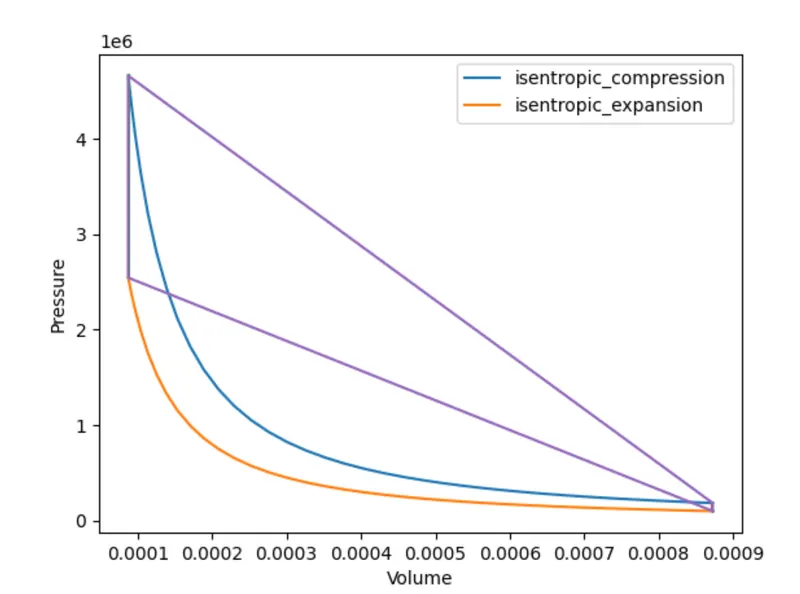
Output:

Conclusion:

• The PV diagram of the Otto cycle has been plotted.
• The air-standard efficiency was found to be 60% for a CR of 10.
• A higher compression ratio leads to a higher air standard efficiency.