Week 5 - Curve fitting

Aim: To perform curve fitting using Python

Objective:
1) To code and obtain graph of cubic and linear functions for C_p data.
2) To get the coefficients of the equations and compare the futted data with the actual data to observe how well the curve fits.
3) To write a code that computes the characterics of the fitted data to check for errors.

Introduction:

Curve fitting is one of the most powerful and most widely used analysis tools in Origin. Curve fitting examines the relationship between one or more predictors (independent variables) and a response variable (dependent variable), with the goal of defining a "best fit" model of the relationship. For algebraic analysis of data, "fitting" usually means trying to find the curve that minimizes the vertical (y-axis) displacement of a point from the curve (e.g., ordinary least squares). However, for graphical and image applications geometric fitting seeks to provide the best visual fit; which usually means trying to minimize the orthogonal distance to the curve.

Linear curve fitting :
Linear curve fitting, or linear regression, is when the data is fit to a straight line. Although there might be some curve to your data, a straight line provides a reasonable enough fit to make predictions.

The first degree polynomial equation

`y = ax+b` is a line with slope a. A line will connect any two points, so a first degree polynomial equation is an exact fit through any two points with distinct x coordinates.

Polynomial curve fitting:
Polynomial curve fitting is when we fit out data to the graph of a polynomial function.
If the order of the equation is increased to a second degree polynomial, the following results:

`y = ax^2 + bx +c`

This will exactly fit a simple curve to three points.

If the order of the equation is increased to a third degree polynomial, the following is obtained:

`y = ax^3 + bx^2 + cx + d`

This will exactly fit four points.

Measurement of the curve characteristics:

After a curve is obtained through curve fitting , there are 4 quantiities which help us define the measurement of goodness of fit criteria which tells us how well a function represents an actual data.
1) The sum of squares due to error (SSE)
2) R - square
3) Adjusted R - Square
4) Root Mean Squared Error (RMSE)

Equations used :

Sum of Squared Errors (SSE): `Sigma(y_i - f(x_i))`

Sum of Squared Errors (SSR) = `Sigma(f(x_i) - Mean)^2`

SST = SSE + SSR

From these terms, `R^2` can be calculated

`R^2 = (SSR)/(SST`

RMSE = `sqrt((SSE)/n`

Python code:

import numpy as np
import matplotlib.pyplot as plt
from scipy.optimize import curve_fit
import math

#----------------------------------
#Linear curve-fitting
#----------------------------------


#defnition of linear function
def linear(t,a,b):
	return a*t+b

def read_file():
	temperature = []
	cp = []
	for line in open('data','r'):
		values = line.split(',')
		temperature.append(float(values[0]))
		cp.append(float(values[1]))

	return [temperature, cp]

temperature, cp = read_file()
popt,pocv = curve_fit(linear,temperature, cp)
fit_cp = linear(np.array(temperature), *popt)

#understanding the characteristics of curve-fit
s = np.sum(cp)
n = len(cp)
mean = s/n

Sum_of_squared_errors = 0
Sum_of_squared_regression = 0

for i in range(n):
	linear_error = cp[i]-fit_cp[i]
	linear_regress = fit_cp[i]-mean
	Sum_of_squared_errors = (Sum_of_squared_errors + np.sum(pow(linear_error,2)))
	Sum_of_squared_regression = (Sum_of_squared_regression + np.sum(pow(linear_regress,2)))

SSE = Sum_of_squared_errors
SSR = Sum_of_squared_regression

SST = SSE + SSR

R_squared = SSR/SST

Root_Mean_Square_Error = math.sqrt(SSE/n)

print('The RMSE for the linear function is :', Root_Mean_Square_Error)
print('The R_squared for the linear function is :', R_squared)

#plot of the obtained data and curve-fit data. 


plt.plot(temperature,cp,color = 'r', linewidth = 1)
plt.plot(temperature,fit_cp,color = 'b', linewidth = 2)
plt.legend(['actual-data', 'curve-fit data'])
plt.xlabel('temperature')
plt.ylabel('cp')

plt.show()


#----------------------------------
#Cubic and quartic curve-fitting
#----------------------------------

# definition of cubic function

def cube(t,a,b,c,d):
	return a*pow(t,3)+b*pow(t,2)+c*pow(t,1)+d

# definition of a quartic function

def quartic(t,a,b,c,d,e):
	return a*pow(t,4)+b*pow(t,3)+c*pow(t,2)+d*t+e

#reading file from folder

def read_file():
	temperature = []
	cp = []
	for line in open('data','r'):
		values = line.split(',')
		temperature.append(float(values[0]))
		cp.append(float(values[1]))

	return [temperature, cp]



temperature, cp = read_file()

#obtaining fit for the cubic function
popt_3,pocv_3 = curve_fit(cube,temperature, cp)
fit_cp_3 = cube(np.array(temperature), *popt_3)


# obtaining fit data for the quartic function
popt_4,pocv_4 = curve_fit(quartic,temperature, cp)
fit_cp_4 = quartic(np.array(temperature), *popt_4)




#understanding characteristics of the cubic curve
s_cubic = np.sum(cp)
n_cubic = len(cp)
mean_cubic = s_cubic/n_cubic

Sum_of_squared_errors_cubic = 0
Sum_of_squared_regression_cubic = 0

for i in range(n_cubic):
	cubic_error = cp[i]-fit_cp_3[i]
	cubic_regress = fit_cp_3[i]-mean_cubic
	Sum_of_squared_errors_cubic = (Sum_of_squared_errors_cubic + np.sum(pow(cubic_error,2)))
	Sum_of_squared_regression_cubic = (Sum_of_squared_regression_cubic + np.sum(pow(cubic_regress,2)))

SSE_cubic = Sum_of_squared_errors_cubic
SSR_cubic = Sum_of_squared_regression_cubic

SST_cubic = SSE_cubic + SSR_cubic

R_squared_cubic = SSR_cubic/SST_cubic

Root_Mean_Square_Error_cubic = math.sqrt(SSE_cubic/n_cubic)

print('The RMSE for the cubic function is :', Root_Mean_Square_Error_cubic)
print('The R_squared for the cubic function is :', R_squared_cubic)

#understanding characteristics of the quartic curve
s_quartic = np.sum(cp)
n_quartic = len(cp)
mean_quartic = s_quartic/n_quartic

Sum_of_squared_errors_quartic = 0
Sum_of_squared_regression_quartic = 0

for i in range(n_quartic):
	quartic_error = cp[i]-fit_cp_4[i]
	quartic_regress = fit_cp_4[i]-mean_quartic
	Sum_of_squared_errors_quartic = (Sum_of_squared_errors_quartic + np.sum(pow(quartic_error,2)))
	Sum_of_squared_regression_quartic = (Sum_of_squared_regression_quartic + np.sum(pow(quartic_regress,2)))

SSE_quartic = Sum_of_squared_errors_quartic
SSR_quartic = Sum_of_squared_regression_quartic

SST_quartic = SSE_quartic + SSR_quartic

R_squared_quartic = SSR_quartic/SST_quartic

Root_Mean_Square_Error_quartic = math.sqrt(SSE_quartic/n_quartic)

print('The RMSE for the quartic function is :', Root_Mean_Square_Error_quartic)
print('The R_squared for the quartic function is :', R_squared_quartic)


#plot of the obtained data vs the actual data for the cubic function
plt.plot(temperature,cp,color = 'r', linewidth = 1)
plt.plot(temperature,fit_cp_3,color = 'b', linewidth = 2)
plt.legend(['actual-data', 'curve-fit data'])
plt.xlabel('temperature')
plt.ylabel('cp')

plt.show()

#plot of the obtained data vs actual data for the quartic function

plt.plot(temperature,cp,color = 'r', linewidth = 1)
plt.plot(temperature,fit_cp_4,color = 'g', linewidth = 2)
plt.legend(['actual-data', 'curve-fit data'])
plt.xlabel('temperature')
plt.ylabel('cp')

plt.show()

Results:

1) Linear function curve: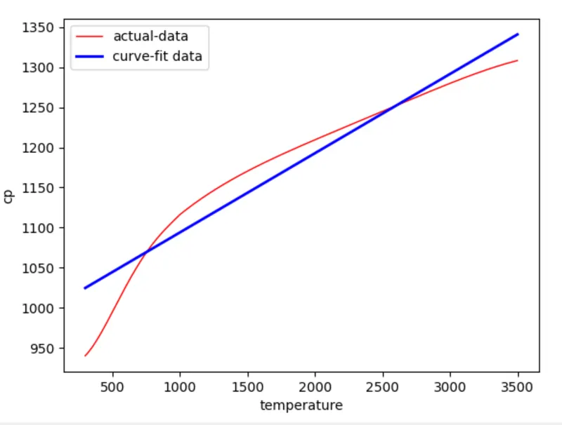

2) Curve for a cubic polynomial: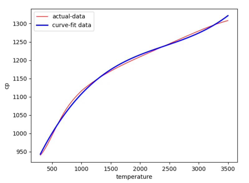

3) Curve for quartic polynomial: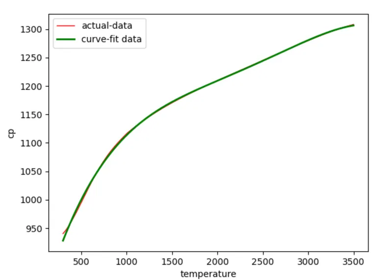

Results of curve characteristics:

RMSE = Root Mean Squared Error

The RMSE for the linear function is : 25.999093068195325
The R_squared for the linear function is : 0.9248776260524184


The RMSE for the cubic function is : 5.42770728878495
The R_squared for the cubic function is : 0.996725946714689


The RMSE for the quartic function is : 1.8599626013389154
The R_squared for the quartic function is : 0.9996155309982948

What does *popt and *pcov mean?
*POPT: popt is a one dimensional array of the best estimates for the parameter values, each entry matches the order in the function definition.

*PCOV: pcov is the covariance matrix showing the uncertainty and interdependence of each parameter in popt.

What does the * in *popt mean?
The '*' value returns each coefficient sotred in the popt array.

What can be done to get a better curve - fit?
If we increase the order of the polynomial, error grows smaller and eventually, we will get a perfect curve-fit.

Conclusion:
From the observed values of errors, as the polynomial order increases, the error decreases.