Study of Mass-Scaling in LS-DYNA
Aim: To study the effect of mass scaling for different values of dt2ms and tssfac.
Procedure: The timestep for any explicit analysis is dependent on the size of the elements in the model. If the timestep of goes below a certain value, there are instabilities produced in the model and hence, explicit analysis is a conditional analysis as opposed to implicit. We can add non-physical mass to elements to make sure the timestep criteria for every element is adhered to. In doing so, we do affect the results of the simulation. There is a certain percentage of mass that is allowed to be added, and in this case, it is 8%. Adding mass to a non-critical area is insignificant in terms of changing the results.
Mass can be artificially added to elements in a selective manner. It is up to a CAE analyst to decide what would be the right percentage. This mass scaling effect to change the minimum timestep to keep the solution intact is done using the DT2MS option in *Control_Timestep.
A positive value of DT2MS will ensure every element has the same mass added or subtracted to have the same timestep. A negative value, on the other hand, will lead to the addition of mass only for the elements that need some mass for the minimum timestep to reach the DT2MS value. In a jist, adding mass to these elements would bring their timestep to DT2MS. This seems like a better option than choosing a positive value since that will increase the computational time needed.
Say we increase the value of dt2ms and reduce the value of TSSFAC such that the product of TSSFAC and DT2MS remains constant, the timestep will remain the same but the mass added will increase.
However, low values of tssfac help with achieving a stable solution. If the solution is not stable with tssfac 0.9, we can try changing the value to 0.8 or 0.7. This again will increase the computational time.
For this experiment, a comparison between the simulation without timestep, with different values of DT2MS is done with TSSFAC being 0.9.
A) Explicit without DT2MS
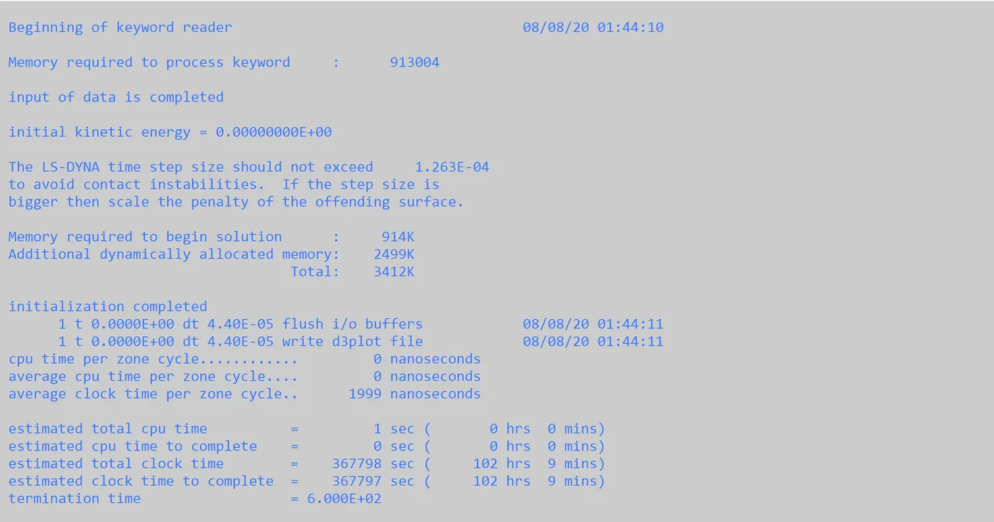
Without DT2MS, the simulation takes around 102 hrs of runtime
B) With DT2MS
Following are the DT2MS values taken for our simulation:
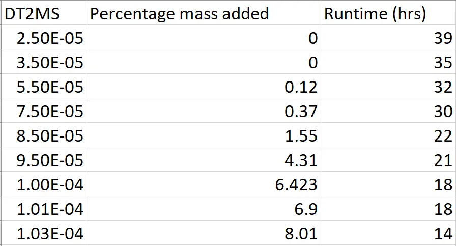
2.5e-5, 3.5e-5, 5.5e-5, 7.5e-5, 8.5e-5, 9.5e-5, 1e-4, 1.01 e-4, 1.029 e-4.
For each value of DT2MS, the amount of mass added is monitored. At 1.029e-4, the amount of mass added is 8% which is the har limit set for mass scaling. Hence, we don't increase the value of DT2MS any further.
Figure: DT2MS = 2.5 e-5
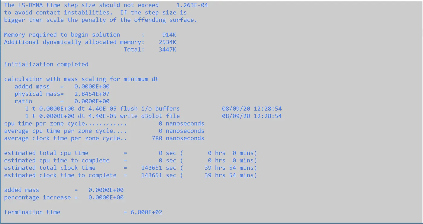
Figure: DT2MS = 3.5e-5
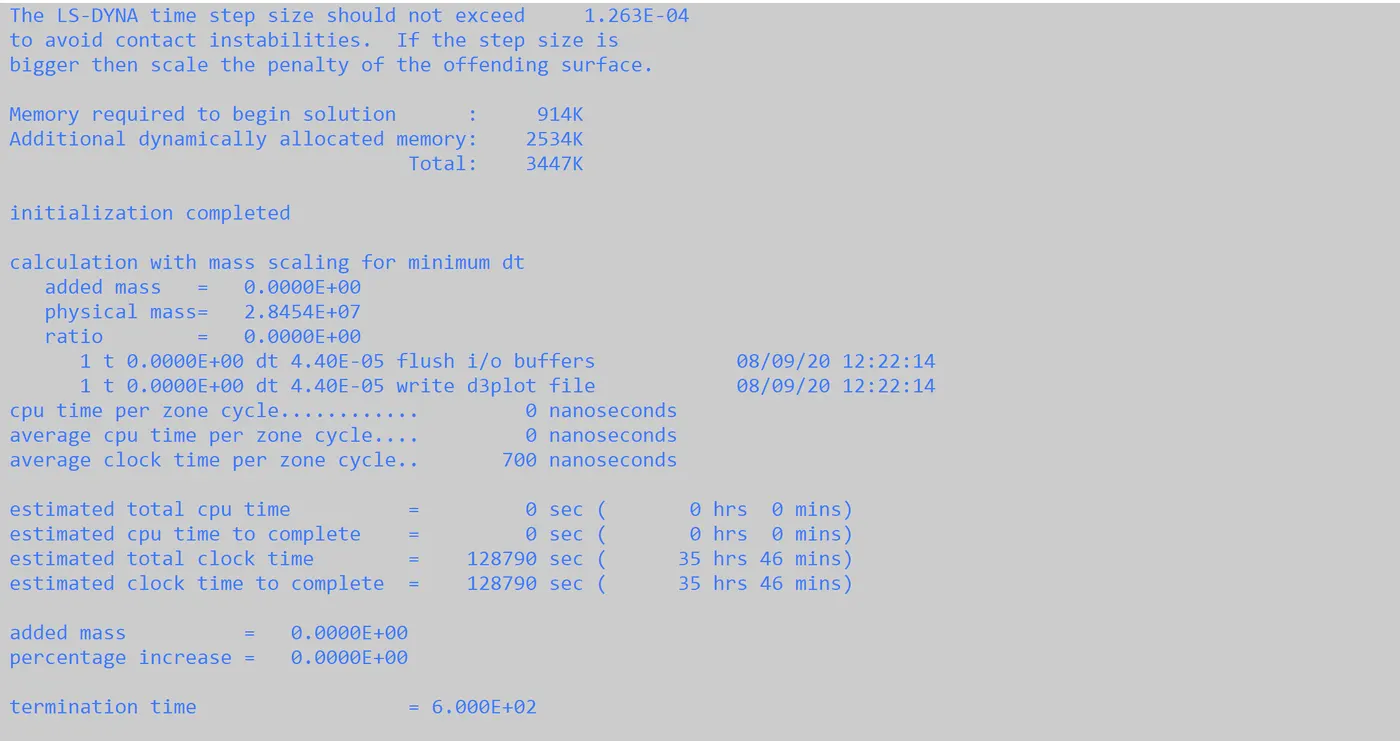
Figure: DT2MS = 7.5e-5
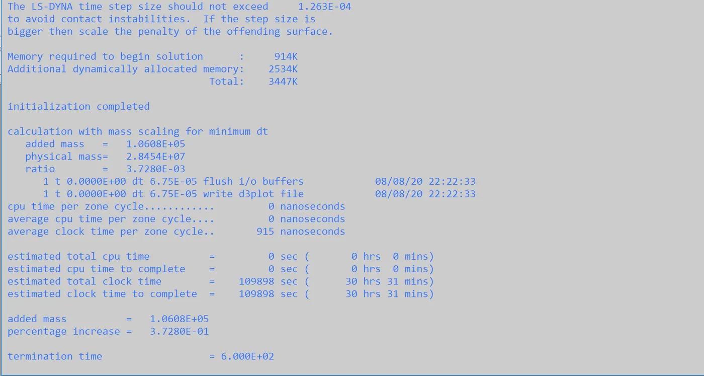
Figure: DT2MS = 9.5e-5
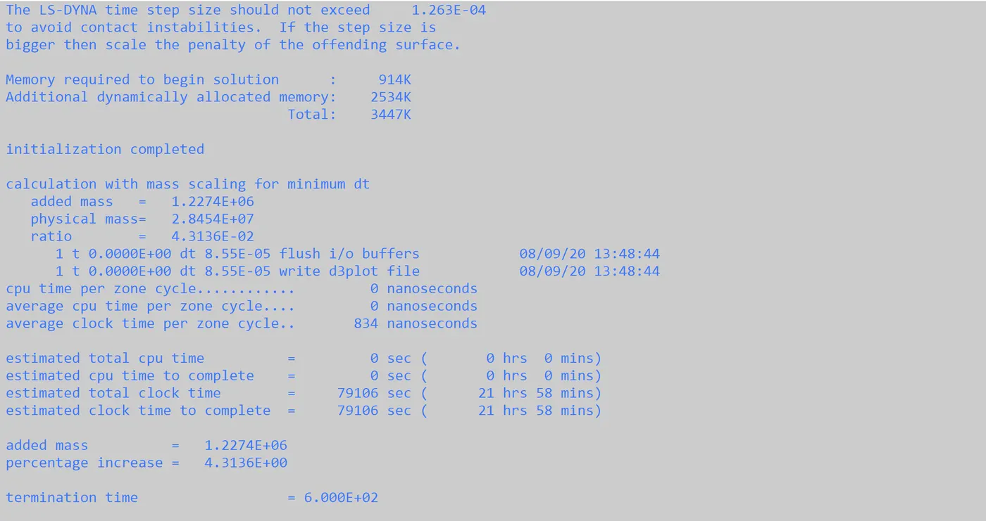
Figure: DT2MS = 1.029e-4
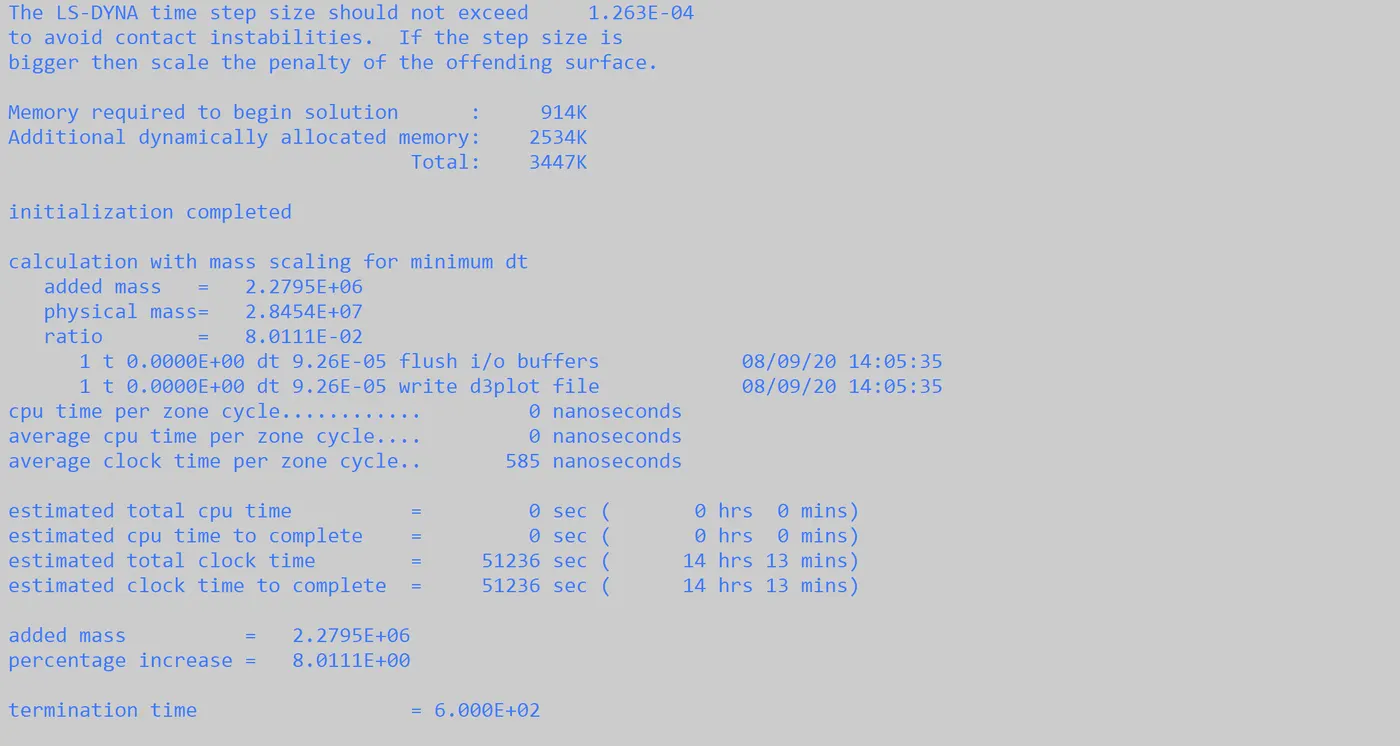
As it can be seen, the mass for dt2ms = 1.029e-4 is exactly 8%
Now, the data below shows the runtime needed for different values of dt2ms along with the mass added for each dt2ms value along with its runtime.
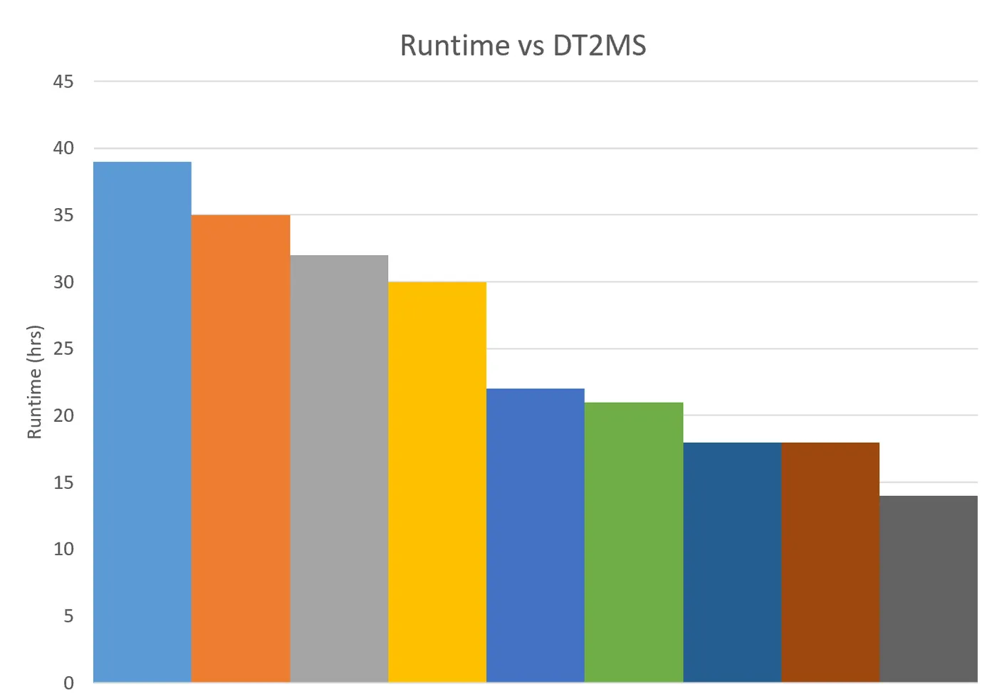
A histogram for the runtime taken for tssface value 0.9 and the dt2ms values as listed above is displayed in the figure below:
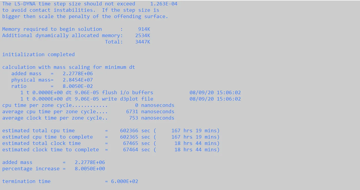
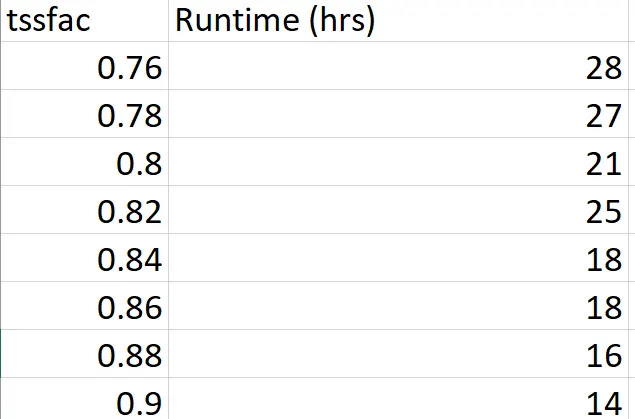
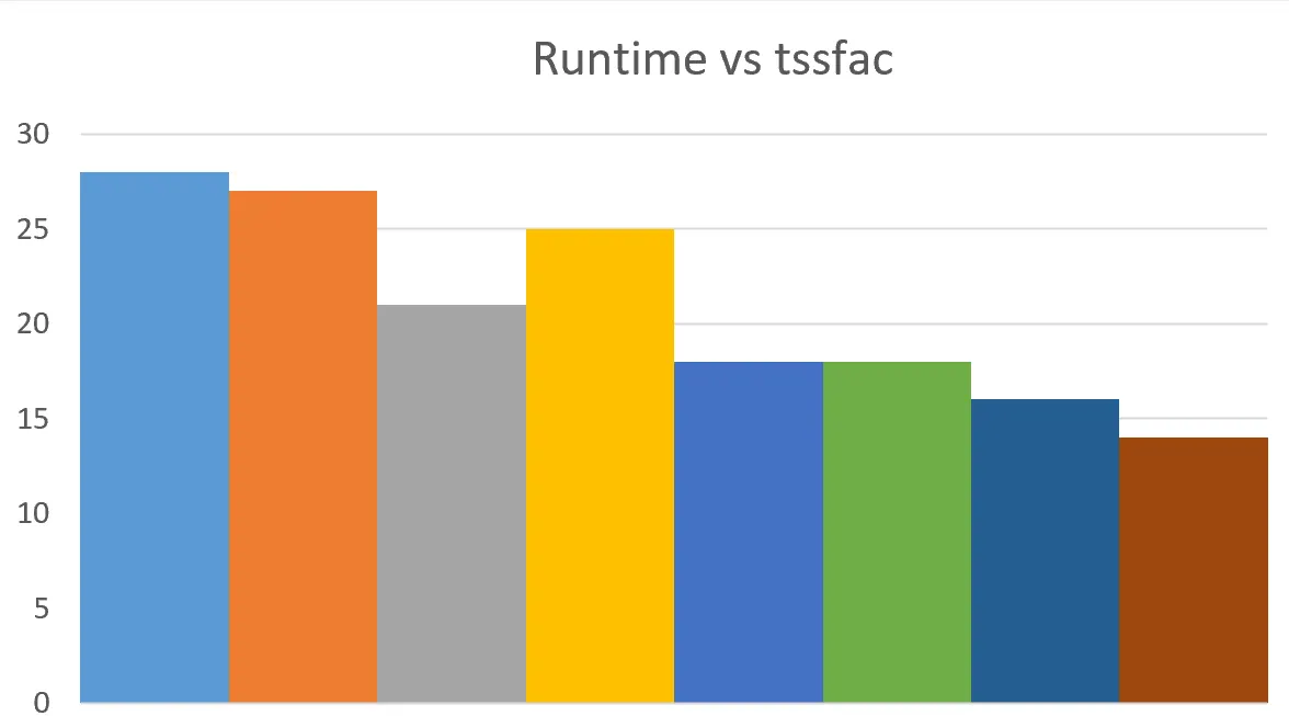
The next step taken was to check the simulation runtime for dt2ms of 1.029e-4 (the point at which mass scaling reaches its limit). The value of tssfac taken were 0.76, 0.78, 0.8, 0.82, 0.84, 0.86, 0.88, 0.9. The general trend of the simulation was a decreasing runtime for increasing values of tssface. However, an anomaly was observed at tssfac of 0.82. This may be because of the computer performance due to background apps that were open which resulted in decrease of performance as opposed to the tssfac effect at all.
Figure: tssfac = 0.76
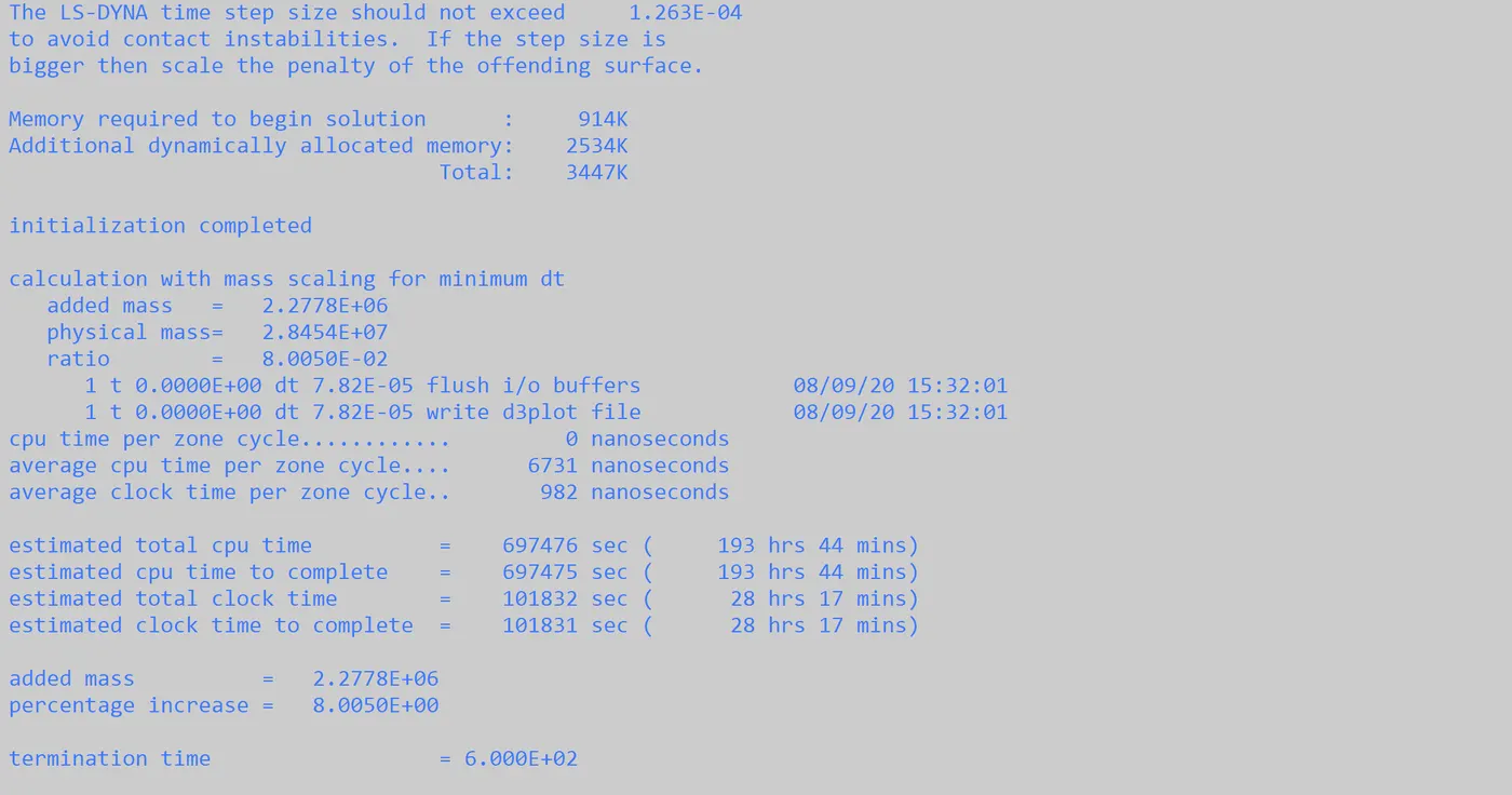
Figure: tssfac = 0.8
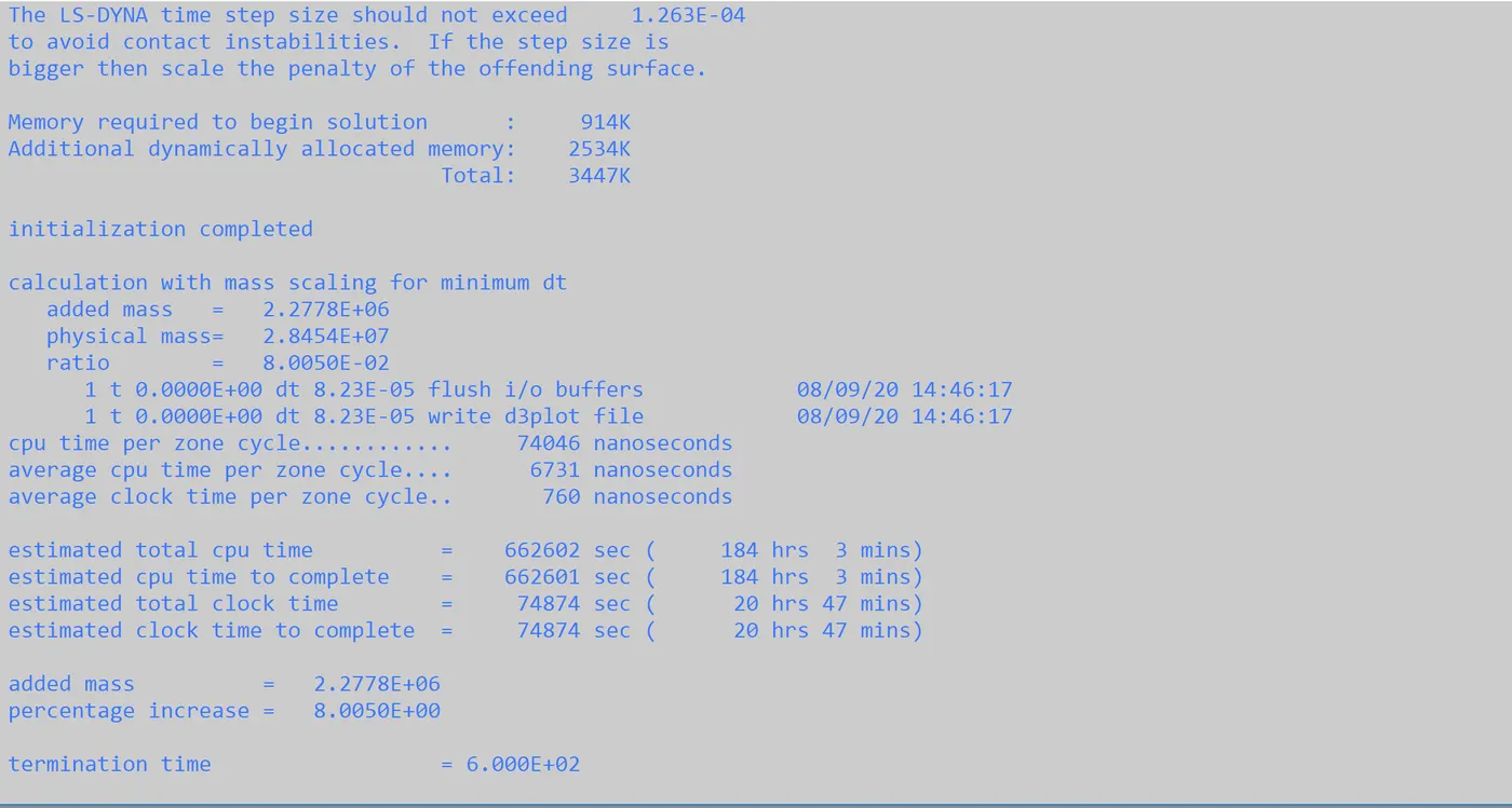
Figure: tssfac = 0.88
The data for the same is shown in the figure below:
The decreasing trend is obvious from the chart below:
Finally, to see how the simulation behaves in terms of runtime with implicit analysis, I set up an implicit analysis using *Control_implicit_general, *Control_implicit_auto, *Control_implicit_solution, *Control_implicit_solver. The initial time is set to 6 ms. In the control_implicit_auto card, the maximum step size used was 5 and the minimum used was 0.01. The iteopt and itewin were set to 11 and 5. And the values for nsolvr in the control_implicit_solution were set to default. Finally, the lsolvr type in control_implicit_solvr was chosen to be 5 (double precision, multi-frontal sparse solver)
The runtime using the above values was 10 mins.
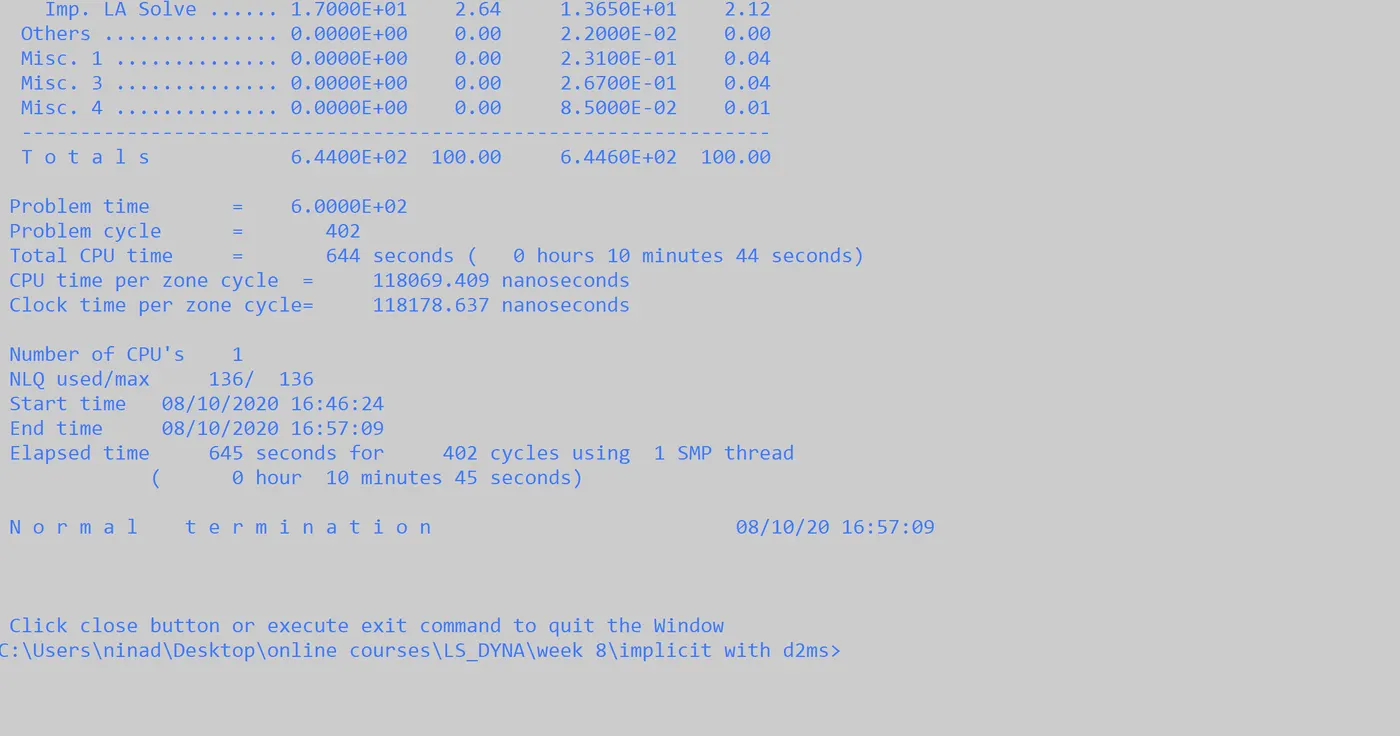
Conclusion: The objective of comparing runtime for a different type of simulation was achieved. The minimum time taken was by the implicit solver. For the explicit type of analysis, the runtime decreased with increasing artificial mass up to 8% as expected.